Radial Electron Probability Density Function of Atoms.

Introduction

In quantum mechanics free particles are described by wave functions which satisfy a wave equation. So, there is a wave-particle duality with a relationship between particle properties (energy, E, and momentum, p) and wave properties (frequency, ν, and wavelength, λ) given by Plank's law (E = h ν) and de Broglie equation (λ = h / p ), both of which involve the Planck's constant, h.

The wave function which determines the motion of a single electron is called orbital, χ(r), and depends on the position vector r. If the one-electron wave function is for an atomic system, it is called an atomic orbital (AO).

The one-electron wave function, χ(r), is interpreted as a “probability amplitude” for the electron. The square modulus of the wave function is interpreted as the “probability density” to find an electron:

ρ(r) = |χ(r)|²

(1)

Quantum mechanics only tells us the probability for some quantum events to occur. The probability to find an electron over all the three-dimensional space is equal to 1, and it is given by the integral of the probability density over ℝ³

∫ ℝ³ ρ(r) d³r = +∞ ∫ 0 |χ(r)|² d³r = 1

(2)

In other words, the previous equation provides the number of electrons and the electronic charge in ℝ³. The product ρ(r) d³r gives the probability of finding the electron in an infinitesimal volume element d³r (or dV). If the components of r are the cartesian coordinates x, y, and z, then the volume element is dV = dx dy dz.

Though most atoms, when they are free, are not spherical, still it may be useful to think of an atom as some sort of fuzzy ball of electrons around a small, central, heavy nucleus. And it easy to extend such a mental picture even to bonded atoms in molecules and crystals. For this reason, it is more convenient to express the electron density in spherical coordinates, r, θ and φ, which are related to the cartesian coordinates x, y and z by the transformation

x = r sin θ cos φ
y = r sin θ sin φ
z = r cos θ

(3)

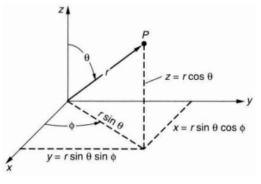
The expression of the density function under the transformation of the random vector variable r is discussed in Section 4.7 of the chapter on "Charge Distributions"“Transformation of the Random Vector Variable”
PAMoC Manual: Charge Distributions, Section 4.7, Equations (4.7.4) and (4.7.10).. The conclusion is that, passing from the reference system of Cartesian axes x, y and z to the reference system of curvilinear coordinates r, θ and φ, the value of the probability density must be multiplied by the determinant of the Jacobian matrix of the transformation of coordinates, which in the case of spherical coordinates is r² sin θ:

ρ(r,θ,φ) = ρ(x,y,z) det | ∂ r ∂ r ∂ r ∂ θ ∂ r ∂ φ |

ρ(r,θ,φ) = ρ(x,y,z) det

sin θ cos φ	r cos θ cos φ	− r sin θ sin φ
sin θ cos φ	r cos θ sin φ	r sin θ cos φ
cos θ	− r sin θ	0

ρ(r,θ,φ) = ρ(x,y,z) r² sinθ

(4)

In general an orbital has the structure

χ_n,ℓ,m(r) = R_n(r) Y_ℓ,m(θ,φ)

(5)

where R_n(r) are radial functions and Y_ℓ,m(θ,φ) are spherical harmonics [L1(a) Wikipedia contributors, "Spherical harmonics,"
Wikipedia, The Free Encyclopedia.
(b) Citizendium contributors, "Spherical harmonics."
Citizendium, The Citizens' Compendium.
(c) Weisstein, E. W. "Spherical Harmonic,"
From MathWorld - A Wolfram Web Resource., L2Wikipedia contributors, "Table of spherical harmonics,"
Wikipedia, The Free Encyclopedia., N1Real Spherical Harmonics.] of degree ℓ and order m. Spherical harmonics can be represented using spherical coordinates (which are convenient when computing integrals) or polynomials (as is commonly done when evaluating them). The integer n = 1, 2, … is the principal quantum number, the integer ℓ = 0, 1, … n − 1 is the azimuthal quantum number, and the integer m = −ℓ, −ℓ + 1, …, ℓ − 1, ℓ is the magnetic quantum number. By virtue of eq. (4) combined with eq. (5), the electron density function in the system of curvilinear coordinates r, θ and φ is given by

(6)

This is the joint probability density“Joint and Marginal Probability Density Function”
PAMoC User's Manual which is related to the probability ρ_n,ℓ,m(r,θ,φ) dr dθ dφ of finding the electron in an infinitesimal volume element, which in spherical coordinatess, is given by dV = r² sinθ dr dθ dφ.[N2Volume element in spherical coordinates.] The joint probability density is factorized into the product of two marginal densities, ρ_n(r) and ρ_ℓ,m(θ,φ) . The marginal density function“Joint and Marginal Probability Density Function”
PAMoC User's Manual ρ_ℓ,m(θ,φ) is defined by

ρ_ℓ,m(θ,φ) = |Y_ℓ,m(θ,φ)|² sinθ

(7)

and is related to the probability ρ_ℓ,m(θ,φ) dθ dφ of finding the electron on a surface element of the unit sphere,[N3Surface area element in spherical coordinates.] i.e. the element of solid angle dΩ = sinθ dθ dφ.[N4Solid angle element in spherical coordinates.]

The radial electron density“Joint and Marginal Probability Density Function”
PAMoC User's Manual ρ_n(r), also referred to as the radial distribution, is defined by

ρ_n(r) = r² |R_n(r)|²

(8)

and is related to the probability ρ_n(r) dr that a measurement of the electron's position yields a value anywhere in a spherical shell of infinitesimal thickness at a distance r from the nucleus as shown in the following figure for the radial distribution with n = 1.[N5Volume of a spherical shell of infinitesimal thickness.]

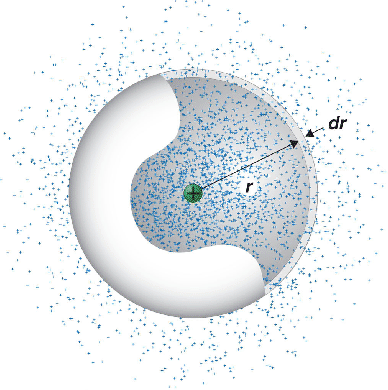
What the radial probability distribution shows is that the electron cannot be sucked into the nucleus because ρ_n(0) = 0. Hence, as we shrink the radial shell into the nucleus, the probability of finding the electron in that shell goes to 0.[L3Mark E. Tuckerman
“The Schrödinger equation for the hydrogen atom and hydrogen-like cations”
2011-10-26.]

The density functions in eqs (7-9) are normalized to 1, meaning that the probability to find the electron in ℝ³ as well as the number of electrons and the electronic charge in ℝ³ are equal to 1.

+∞ ∫ r=0 π ∫ θ=0 2π ∫ φ=0 ρ_n,ℓ,m(r,θ,φ) dr dθ dφ = +∞ ∫ r=0 π ∫ θ=0 2π ∫ φ=0 | χ_n,ℓ,m(r,θ,φ) |² r² sinθ dr dθ dφ = 1

(9)

π ∫ θ=0 2π ∫ φ=0 ρ_ℓ,m(θ,φ) dθ dφ = π ∫ θ=0 2π ∫ φ=0 |Y_ℓ,m(θ,φ)|² sinθ dθ dφ = 1

(10)

+∞ ∫ r=0 ρ_n(r) dr = +∞ ∫ r=0 r² |R_n(r)|² dr = 1

(11)

The normalization property of the radial density function, eq. (11), is strictly related to the radial cumulative distribution function D_n(r), which is defined as the probability to find the electron in the interval [0,r] and has the following expression

D_n(r) = r ∫ 0 ρ_n(r') dr' = r ∫ 0 r'² |R_n(r')|² dr'

(12)

(see section 4.2 of the chapter on “Charge Distributions” for more details). It satisfies the relationships D(0) = 0, lim_r→+∞ D(r) = 1, and dD(r) / dr = ρ(r). In addition, the probability to find the electron in any interval [a,b] (∀ 0 ≤ a < b ∈ ℝ) is given by the difference D(b) − D(a). The joint cumulative distribution functions D_n,ℓ,m(r,θ,φ) and D_ℓ,m(θ,φ) are defined in a similar way.

Explicit expressions for normalized Slater-type orbitals (STO) and Gaussian-type orbitals (GTO) in spherical coordinates and in Cartesian coordinates are given in reference [1Gomes, A. S. P.; Custodio, R.
J. Comput. Chem. 2002, 23, 1007-1012.] (click to view/hide details).

They are also compared in the following table.

**Normalized Slater-type orbitals (STO) and Gaussian-type orbitals (GTO) in spherical coordinates and Cartesian coordinates.**[1Gomes, A. S. P.; Custodio, R.
*J. Comput. Chem.* **2002**, 23, 1007-1012.]
	Spherical STO	Spherical GTO
Orbital	χ_n,ℓ,m(ζ; r,θ,φ) = R_n(ζ; r) Y_ℓ,m(θ,φ)	χ_n,ℓ,m(α; r,θ,φ) = R_n(α; r) Y_ℓ,m(θ,φ)	(D1)
Radial function	R_n(ζ; r) = N_n(ζ) rⁿ⁻¹ e^−ζr	R_n(α; r) = N_n(α) rⁿ⁻¹ e^−αr²	(D2)
Normalizing constant	N_n(ζ) = [ (2ζ)²ⁿ⁺¹ / (2n)! ]^{^{^¹⁄₂}}	N_n(α) = [ 2⁴ⁿ⁺³ α²ⁿ⁺¹ / [(2n − 1)!!]² π ]^{^{^¹⁄₄}}	(D3)
	Cartesian STO	Cartesian GTO
Orbital	χ_a,b,c,k(ζ; x,y,z) = N_a,b,c,k(ζ) x^a y^b z^c r^k−1 e^−ζr	χ_a,b,c(α; x,y,z) = N_a,b,c(α) x^a y^b z^c e^−αr²	(D4)
Normalizing constant	N_a,b,c,k(ζ) = [ (2ζ)^2k+1 / (2k)! (2a + 2b + 2c + 1)!! / 4π (2a − 1)!! (2b − 1)!! (2c − 1)!! ]^{^{^¹⁄₂}}	N_a,b,c(α) = [ 2^{2(a + b + c) + ³⁄₂} α^{a + b + c + ³⁄₂} / π^³⁄₂ (2a − 1)!! (2b − 1)!! (2c − 1)!! ]^{^{^¹⁄₂}}	(D5)

where n, ℓ, and m are the well-known quantum numbers, in addition k = n − (a + b + c) and a, b, and c are integers. The sum a + b + c = ℓ is usually referred to as s, p, d, etc., even though they generally contain components of lower angular momentum. The functions Y_ℓ,m(θ,φ) are orthonormalized real spherical harmonics. Their expressions can be found in reference [L2Wikipedia contributors, "Table of spherical harmonics,"
Wikipedia, The Free Encyclopedia.].

Derivation of the normalization constants can be found on the tutorial pages of this manual (Exercise 1, Exercise 2, Exercise 3, Exercise 4, Exercise 5).

A simple case: the ground state of the hydrogen atom

The Schrödinger equation (in atomic units) for the hydrogen atom is[2Szabo, A.; Ostlund, N. S.
“Modern Quantum Chemistry - Introduction to Advanced Electronic Structure Theory”
Macmillan Publishing Co., Inc., New York, 1982, p. 33.]

(− 1 2 ∇² − Z r ) ❘Φ⟩ = E ❘Φ⟩

(13)

where Z is the atomic number and is equal to the nuclear charge. The same equation also applies to hydrogen-like (or hydrogenic) ions, which are constituted by any atomic nucleus with a single electron, so that they are isoelectronic with hydrogen. These ions carry the positive charge (Z − 1) e, where Z is the atomic number of the atom. Left multiplying both sides of eq. (13) by ⟨Φ❘, yields the formal solution

E_1s = ⟨ Φ❘− 1 2 ∇² − Z r ❘Φ ⟩ ⟨Φ❘Φ⟩

(14)

If we use the 1s-STO ❘Φ⟩ ≡ χ_1,0,0(r) = R₁(r) Y_0,0(θ,φ) as a trial function for the ground state energy of the hydrogen atom, eq. (14) can be rewritten as

E_1s = ⟨ R₁(r)❘− 1 2 ∇² − Z r ❘R₁(r) ⟩ ⟨ Y_0,0(θ,φ) ❘ Y_0,0(θ,φ) ⟩ ⟨Φ❘Φ⟩

(15)

Both the radial part, R₁(r), and the angular part, Y_0,0(θ,φ), of the 1s-STO χ_1,0,0(r) as well as the 1s-STO itself are normalized separately, i.e.

⟨Y_0,0(θ,φ)❘Y_0,0(θ,φ)⟩ = 1 4 π π ∫ 0 sinθ dθ 2π ∫ 0 dφ
⟨Y_0,0(θ,φ)❘Y_0,0(θ,φ)⟩ = 1 4 π ⋅ [−cosθ ]^{^{^π}}₀ ⋅ [φ ]^{^{^2π}}₀
⟨Y_0,0(θ,φ)❘Y_0,0(θ,φ)⟩ = 1 4 π ⋅ 2 ⋅ 2 π = 1

(16)

where the spherical harmonic of degree ℓ = 0 and order m = 0 is the constant Y₀₀ = 1 / 2 √ 1 / π , [L2Wikipedia contributors, "Table of spherical harmonics,"
Wikipedia, The Free Encyclopedia.]

⟨R₁(r)❘R₁(r)⟩ = 4 ζ³ +∞ ∫ 0 e^{−2ζ r} r² dr = 4 ζ³ ⋅ 1 4 ζ³ = 1

(17)

where the radial part of the 1s-STO has the expression R₁(r) = 2 √ζ³ e^{−ζ r} (cf the table in the “details” section above), and

⟨Φ❘Φ⟩ ≡ ⟨χ_1,0,0(r)❘χ_1,0,0(r)⟩ = ⟨R₁(r)❘R₁(r)⟩ ⟨Y_0,0(θ,φ)❘Y_0,0(θ,φ)⟩ = 1

(18)

where the 1s-STO has the espression χ_1,0,0(r) = √ ζ³ / π e^{−ζ r}.

Substituting the Laplace operator ∇² in eq. (15) with its expression in spherical coordinates, and remembering the normalization conditions (16-18), yields

E_1s = ⟨ R₁(r)❘− 1 2 d² d r² − 1 r d d r − Z r ❘R₁(r) ⟩
E_1s = ⟨ R₁(r)❘− ζ² 2 − 1 r (Z − ζ) ❘R₁(r) ⟩
E_1s = − ζ² 2 ⟨R₁(r)❘R₁(r)⟩ + (ζ − Z) ⟨ R₁(r)❘ 1 r ❘R₁(r) ⟩
E_1s = − ζ² 2 + 4 ζ³ (ζ − Z) +∞ ∫ 0 r e^{−2ζ r} dr
E_1s = − ζ² 2 + 4 ζ³ (ζ − Z) 1 (2 ζ)²
E_1s = − ζ² 2 + ζ (ζ − Z)

(19)

In deriving eqs (17) and (19) use of the integral +∞ ∫ 0 rⁿ e^{−γ r} dr = n! / γⁿ⁺¹ has been made [3“A Concise Handbook of Mathematics, Physics, and Engineering Sciences”
Polyanin, A. D., Chernoutsan, A. I., Eds.
Taylor & Francis Group: New York, 2011.] (cf the Exercise 2 to see how the integral can be worked out). The optimal value of the Slater exponent ζ is determined by calculating the energy derivative with respect to ζ and equating to zero, i.e.

d E_1s d ζ = ζ − Z = 0 ⇒ ζ = Z

so that eq. (19) yields

E_1s = − Z² 2

(20)

The radial density function of the ground state of the hydrogen atom is given by eq.(8) with n = 1, i.e.

ρ_1s(r) = r² |R(r)|² = 4 ζ³ r² e^{− 2 ζ r}

(21)

STOs with n ≥ 1 differ significantly from the exact solutions of eq. (13) for hydrogenic atoms.[4Leonard I. Schiff
“Quantum Mechanics”
McGraw-Hill, 1968, Chapter 16, pp. 88-99., 5Paul A. Tipler and Gene Mosca
“Physics for Scientists and Engineers: Extended Version”.
W. H. Freeman, 2003, Section 36-4, p. 1181., 6David A. B. Miller
“Quantum Mechanics for Scientists and Engineers”
Cambridge University Press, 2008, Chapter 10, pp. 259-278., L6Citizendium contributors
“Hydrogen-like atom”
Citizendium, The Citizens' Compendium.] The largest difference is the absence of nodes in the radial dependence of the wavefunction (click to view/hide details).

Solving the Schrodinger equation with the radial function

R_n(r) = [ (2ζ)²ⁿ⁺¹ (2n)! ]^{^{^¹⁄₂}} rⁿ⁻¹ e^{−ζ r}

as a trial function yields

E_ns = ⟨ R_n(r)❘− 1 2 d² d r² − 1 r d d r − Z r ❘R_n(r) ⟩
E_ns = ⟨ R_n(r)❘− ζ² 2 + n ζ − Z r − n (n − 1) 2 r² ❘R_n(r) ⟩
E_ns = − ζ² 2 ⟨R_n(r)❘R_n(r)⟩ + (n ζ − Z) ⟨R_n(r)❘r⁻¹❘R_n(r)⟩ − n (n − 1) 2 ⟨R_n(r)❘r⁻²❘R_n(r)⟩

where

⟨R_n(r)❘R_n(r)⟩ = 1

⟨R_n(r)❘r⁻¹❘R_n(r)⟩ = (2ζ)²ⁿ⁺¹ (2n)! +∞ ∫ 0 r²ⁿ⁻¹ e^{−2ζ r} dr = (2ζ)²ⁿ⁺¹ (2n)! ⋅ (2 n − 1)! (2 ζ)²ⁿ = ζ n

⟨R_n(r)❘r⁻²❘R_n(r)⟩ = (2ζ)²ⁿ⁺¹ (2n)! +∞ ∫ 0 r²ⁿ⁻² e^{−2ζ r} dr = (2ζ)²ⁿ⁺¹ (2n)! ⋅ (2 n − 2)! (2 ζ)²ⁿ⁻¹ = 2 ζ² n (2n − 1)

so that

E_ns = − ζ² 2 + ζ (n ζ − Z) n − (n − 1) ζ² 2n − 1
E_ns = ζ [n ζ − 2 (2n − 1) Z] 2 n (2n − 1)

Differentiating with respect to ζ and equating to zero yields

d E_ns d ζ = n ζ − (2n − 1) Z n (2n − 1) = 0 ⇒ ζ = 2n − 1 n Z

so that

E_ns = − Z² 2 n² (2n − 1)

which overestimates the exact value by a factor of (2n − 1). The exact solution of eq (13) is expressed in terms of hydrogenic orbitals

ψ_n,ℓ,m(α; r,θ,φ) = R_n,ℓ(α; r) Y_ℓ,m(θ,φ)

where Y_ℓ,m(θ,φ) are spherical harmonics [L1(a) Wikipedia contributors, "Spherical harmonics,"
Wikipedia, The Free Encyclopedia.
(b) Citizendium contributors, "Spherical harmonics."
Citizendium, The Citizens' Compendium.
(c) Weisstein, E. W. "Spherical Harmonic,"
From MathWorld - A Wolfram Web Resource., L2Wikipedia contributors, "Table of spherical harmonics,"
Wikipedia, The Free Encyclopedia., N1Real Spherical Harmonics.] of degree ℓ and order m. The functions R_n,ℓ(α; r) describe the radial dependence of the wavefunction

R_n,ℓ(α; r) = N_n,ℓ(α) ( 2Z r n ) ^{^{^{^ℓ}}} L^2ℓ+1_n−ℓ−1 ( 2Z r n ) exp ( − Z r n )

where L^2ℓ+1_n−ℓ−1 ( 2Z r n ) is a Laguerre polynomial. The normalization constant N_n,ℓ(α) is given by

N_n,ℓ(α) = √ (n − ℓ − 1)! 2n (n + ℓ)! ( 2Z n ) ^{^{^³}}

STOs, introduced in 1930 by Slater,[Slater J C 1930 Phy. Rev. 36 57] are defined as

χ_n,ℓ,m(ζ; r,θ,φ) = R_n(ζ; r) Y_ℓ,m(θ,φ)

where the radial function R_n(ζ; r) does not depend on the azimuthal quantum number ℓ and on the Laguerre polynomial, implying the absence of nodes, as can be seen by its explicit expression

R_n(ζ; r) = N_n(ζ) rⁿ⁻¹ e^{−ζ r}

^(a) The radial function depends on both the quantum numbers n and ℓ. ^(b) The one-dimensional Schrödinger equation for the radial distance r is solved by finding the behavior at large r, then finding the behavior at small r, and then using the trial function

R(s) = s^ℓ L(s) exp(−s/2)

where the variable s = 2Z r n is a scaled radial distance and L(s) is actually the function to be determined. It can be described as a power series whose coefficients turn out to be those of a standard set of known polynomials, the associated Laguerre polynomials which, in the notation of Abramowitz and Stegun,[7Milton Abramowitz and Irene A. Stegun, eds.
“Handbook of Mathematical Functions with Formulas, Graphs, and Mathematical Tables”.
New York: Dover, 1972, § 22.3, p. 775.] are defined as

L^j_p(s) = p ∑ q=0 (−1)^q ( p + j p − q ) 1 q! s^q = p ∑ q=0 (−1)^q (p + j)! (p − q)! (j + q)! q! s^q

with p = n − ℓ − 1 and j = 2ℓ + 1. The radial wavefunction R_n,ℓ(r) obeys the normalization condition

[N_n,ℓ]² +∞ ∫ 0 [R_n,ℓ(r)]² r² dr ≡ [N_n,ℓ]² ( n 2Z ) ^{^{^³}} +∞ ∫ 0 [R_n,ℓ(s)]² s² ds = 1

where the identity r = n 2Z s has been used. It is possible to show that

+∞ ∫ 0 [R_n,ℓ(s)]² s² ds = +∞ ∫ 0 s^2ℓ [L^2ℓ+1_n−ℓ−1(s) ]² e^−s s² ds = 2n (n + ℓ)! (n − ℓ − 1)!

from which it can be concluded that the normalization constant of the radial wavefunction is

N_nℓ = √ (n − ℓ − 1)! 2n (n + ℓ)! ( 2Z n ) ^{^{^³}}

^(c) The number of zeros in the wavefunction is n − 1. The associated Laguerre polynomials in the radial wavefunction have n − ℓ − 1 zeros, and the spherical harmonics have ℓ nodal “circles”.
^(d) ζ = 2n − 1 n Z.

Table - Comparison of various low order radial wavefunctions of hydrogenic atoms with the corresponding STO approximations.

R_nℓ

exact hydrogenic orbital^(a-c)
R_nℓ(r) = √ (n − ℓ − 1)! 2n (n + ℓ)! ( 2Z n ) ^{^{^³}} ( 2Z r n ) ^{^{^{^ℓ}}} L^2ℓ+1_n−ℓ−1 ( 2Z r n ) exp ( − Z r n )

STO approximation
R_n(r) = √ (2ζ)²ⁿ⁺¹ (2n)! rⁿ⁻¹ e^{−ζ r}

R_1,0 ≡ R_1s

2 √Z³ e^{−Z r}

R_2,0 ≡ R_2s

√2 Z³ 4 (2 − Z r) e^{−Z r/2}

9 √2 Z⁵ 4 r e^{−3Z r/2}

R_2,1 ≡ R_2p

√6 Z⁵ 12 r e^{−Z r/2}

R_3,0 ≡ R_3s

2 √3 Z³ 27 (3 − 2Z r + 2 9 Z² r² ) e^{−Z r/3}

250 √6 Z⁷ 243 r² e^{−5Z r/3}

R_3,1 ≡ R_3p

√6 Z⁵ 81 r (4 − 2 3 Z r ) e^{−Z r/3}

R_3,2 ≡ R_3d

2 √30 Z⁷ 1215 r² e^{−Z r/3}

R_4,0 ≡ R_4s

√Z³ 16 (4 − 3Z r + 1 2 Z² r² − 1 48 Z³ r³ ) e^{−Z r/4}

2401 √5 Z⁹ 3840 r³ e^{−7Z r/4}

R_4,1 ≡ R_4p

√15 Z⁵ 192 r (4 − Z r + 1 20 Z² r² ) e^{−Z r/4}

R_4,2 ≡ R_4d

√5 Z⁷ 3840 r² (12 − Z r) e^{−Z r/4}

R_4,3 ≡ R_4f

√35 Z⁹ 26880 r³ e^{−Z r/4}

Exercise: Find the moment generating function of an exponential random variable r with parameter ζ, e.g. the radial density function of the gound state of the hydrogen atom (click to view/hide details).

If the radial density function of the ground state of the hydrogen atom is ρ(r) = γ³ 2 r² e^{−γ r}, where γ = 2 ζ, the moment generating function is by definition:

M_r(s) = E(e^{s r}) = +∞ ∫ 0 e^{s r} ρ(r) dr = γ³ 2 +∞ ∫ 0 e^−(γ−s)r r² dr = γ³ (γ − s)³

provided that s < γ. Note that M_r(s)❘_s=0 = 1 is the normalization condition of the radial density function ρ(r). It's now easy to verify that the n-th derivative of M_r(s) with respect to s (n times),

dⁿ d sⁿ M_r(s) = dⁿ d sⁿ [γ (γ − s)⁻¹]³ = n! 2 (γ − s)ⁿ

calculated at s = 0, equals the n-th moment of ρ(r):

dⁿ d sⁿ M_r(s)❘_s=0 = n! 2 γⁿ.

Indeed, the n-th moment of ρ(r) is by definition:

⟨rⁿ⟩ ≡ E(rⁿ) = +∞ ∫ 0 rⁿ ρ(r) dr = γ³ 2 +∞ ∫ 0 e^{−γ r} rⁿ⁺² dr = n! 2 γⁿ.

Exercise: Use an 1s-GTO, as a trial function, to find an upper bound to the exact ground state energy of the hydrogen atom (click to view/hide details).

An 1s-GTO has the form

❘Φ⟩ = ( 2α π )^{^{^³⁄₄}} e^{−α r²}

(t)

and satisfies the normalization condition, ⟨Φ❘Φ⟩ = 1, i.e.

⟨Φ❘Φ⟩ = ( 2α π )^{^{^³⁄₂}} +∞ ∫ 0 e^{−2α r²} r² dr π ∫ 0 sinθ dθ 2π ∫ 0 dφ
⟨Φ❘Φ⟩ = ( 2α π )^{^{^³⁄₂}} ⋅ π^½ 4 (2 α)^{^3/2} ⋅ 4 π = 1

(u)

The ground state energy, eq.(14), is then given by

E = ⟨ Φ❘− 1 2 d² d r² − 1 r d d r − Z r ❘Φ ⟩ = ⟨ Φ❘− 2 α² r² + 3 α − Z r ❘Φ ⟩
E = 4 π ( 2α π )^{^{^³⁄₂}} ( − 2 α² +∞ ∫ 0 e^{−2α r²} r⁴ dr + 3 α +∞ ∫ 0 e^{−2α r²} r² dr − Z +∞ ∫ 0 r e^{−2α r²} dr )
E = 4 π ( 2α π )^{^{^³⁄₂}} [ 3 16 ( π 2 α )^{^{^¹⁄₂}} − Z 4 α ]
E = 1 2 ( 3 α − 8 Z √ α 2 π )

(v)

where the values of the following definite integrals,[3“A Concise Handbook of Mathematics, Physics, and Engineering Sciences”
Polyanin, A. D., Chernoutsan, A. I., Eds.
Taylor & Francis Group: New York, 2011.] +∞ ∫ 0 r²ⁿ e^{−γ
r²} dr = (2 n − 1)!! 2ⁿ⁺¹ γⁿ ( π γ )^{^{^¹⁄₂}} = (2 n)! 2²ⁿ⁺¹ n! γⁿ ( π γ )^{^{^¹⁄₂}} and +∞ ∫ 0 r²ⁿ⁺¹ e^{−γ
r²} dr = n! 2 γⁿ⁺¹ , have been used. The optimal value of the exponent α is obtained by solving the equation d E d α = 0, i.e.

3 − 4 Z √ 2 π α = 0 ⇒ α = 8 Z² 9 π = 0.28294246 Z²

(w)

Back substituting this value of the exponent α into the last equality of eq. (v) we find that E = − 4 Z² 3 π = −0.42441369 Z² hartree is an upper bound to the exact ground state energy (which is -0.5 hartree).[2Szabo, A.; Ostlund, N. S.
“Modern Quantum Chemistry - Introduction to Advanced Electronic Structure Theory”
Macmillan Publishing Co., Inc., New York, 1982, p. 33.] Finally, the normalization constant becomes

( 2α π )^{^{^³⁄₄}} = 8 ( Z 3 π )^{^{^³⁄₂}} = 0.27649271 Z^3/2

(x)

and the adial density function of the ground state of the hydrogen atom is

ρ_1s(r) = 64 27 ( Z π )^{^³} r² exp ( − 16 Z² 9 π r² )

(y)

Exercise: Write the wave function files (.wfn) for the hydrogen atom using both Slater and Gaussian basis sets (click to view/hide details).

1) Slater basis set (a single 1s orbital, according to eq.16):


Name  H     Run Type  SinglePoint    Method  ROHF     Basis Set  Slater
SLATER                1 MOL ORBITALS      1 PRIMITIVES        1 NUCLEI
  H         (CENTRE  1)   0.00000000  0.00000000  0.00000000  CHARGE =  1.0
CENTRE ASSIGNMENTS    1
TYPE ASSIGNMENTS      1
EXPONENTS  1.0000000E+00
MO  1                     OCC NO =   1.00000000 ORB. ENERGY =  -0.5
  0.56418958E+00
END DATA
 THE SCF ENERGY =     -0.500000000000 THE VIRIAL(-V/T)=   2.00000000

2) Gaussian basis set (a single 1s orbital, according to eq.D?):


Name  H     Run Type  SinglePoint    Method  ROHF     Basis Set  STO-1G
GAUSSIAN              1 MOL ORBITALS      1 PRIMITIVES        1 NUCLEI
  H         (CENTRE  1)   0.00000000  0.00000000  0.00000000  CHARGE =  1.0
CENTRE ASSIGNMENTS    1
TYPE ASSIGNMENTS      1
EXPONENTS  0.2829425E+00
MO  1                     OCC NO =   1.00000000 ORB. ENERGY =  -0.42441369
  0.27649271E+00
END DATA
 THE SCF ENERGY =     -0.424413690000 THE VIRIAL(-V/T)=   2.00000000

References

“Exact Gaussian Expansions of Slater-Type Atomic Orbitals”
Gomes, A. S. P.; Custodio, R. J. Comput. Chem. 2002, 23, 1007-1012.
Szabo, A.; Ostlund, N. S. “Modern Quantum Chemistry − Introduction to Advanced Electronic Structure Theory” Macmillan Publishing Co., Inc., New York, 1982, p. 33. ISBN 0-02-949710-8.
“A Concise Handbook of Mathematics, Physics, and Engineering Sciences”; Polyanin, A. D., Chernoutsan, A. I., Eds.; Taylor & Francis Group: New York, 2011.
Leonard I. Schiff, “Quantum Mechanics”. McGraw-Hill, 1968, Chapter 16, pp. 88-99. ISBN-13: 9780070856431. ISBN-10: 0070856435.
Paul A. Tipler; Gene Mosca; “Physics for Scientists and Engineers: Extended Version”. W. H. Freeman, 2003, Section 36-4, p. 1181. ISBN-13: 9780716743897. ISBN-10: 0716743892.
David A. B. Miller, “Quantum Mechanics for Scientists and Engineers”. Cambridge University Press, 2008, Chapter 10, pp. 259-278. ISBN-13: 9780521897839. ISBN-10: 0521897831.
Milton Abramowitz and Irene A. Stegun, eds. “Handbook of Mathematical Functions with Formulas, Graphs, and Mathematical Tables”. United States Government Printing Office, 1972, § 22.3, p. 775. ISBN-13: 9780318117300. ISBN-10: 0318117304.
A. V. Arecchi, T. Messadi, and R. J. Koshel, “Field Guide to Illumination”, SPIE Press, Bellingham, WA, 2007, p. 2. ISBN: 9780819467683.

Notes

Real Spherical Harmonics. Orthonormalized Laplace’s spherical harmonics are defined as

Y_ℓ^m(θ,φ) = (−1)^m N_ℓm P_ℓ^m(cosθ) e^imφ

(N1.1)

where P_ℓ^m(cosθ) is the associate Legendre polynomial of degree ℓ and order m ( ℓ ≥ 0 and −ℓ≤ m ≤ ℓ). Spherical harmonics are single-valued, smooth (infinitely differentiable), complex functions of two variables, θ and φ, indexed by two integers, ℓ and m, and form a complete set of orthonormal functions:

2π ∫ 0 dφ π ∫ 0 Y_ℓ^m(θ,φ) Y_ℓ'^m'*(θ,φ) sinθ dθ = δ_ℓℓ' δ_mm'

(N1.2)

This normalization is used in quantum mechanics because it ensures that probability is normalized, i.e. π ∫ 0 |Y_ℓ^m(Ω)|² dΩ = 1, with dΩ = sinθ dθ and normalization factor:

N_ℓm = √ 2ℓ + 1 4 π ⋅ (ℓ − |m|)! (ℓ + |m|)!

(N1.3)

The real forms of the spherical harmonics, also known as tesseral harmonics, are obtained by taking the linear combinations [Y_ℓ^m(θ,φ) ± Y_ℓ^−m(θ,φ)]/√2. They are defined as follows

Y_ℓm(θ,φ) = M_ℓm U_ℓm(θ,φ)

(N1.4)

where

U_ℓm(θ,φ) = P_ℓ^|m|(cosθ) { cos(|m|φ), m ≥ 0 sin(|m|φ), m < 0

(N1.5)

are the un-normalized tesseral harmonics, and M_ℓm is the normalization factor

M_ℓm = N_ℓm √ 2 − δ_|m|,0 = √ 2ℓ + 1 4 π ⋅ (2 − δ_|m|,0) ⋅ (ℓ − |m|)! (ℓ + |m|)!

(N1.6)

Volume element in spherical coordinates.

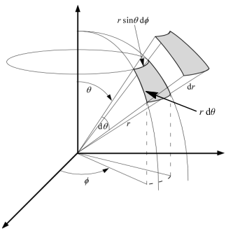
Working in spherical coordinates, the diagram on the left enable us to calculate the infinitesimal volume element as

dV = dr ⋅ r dθ ⋅ r sinθ dφ = r² sinθ dr dθ dφ

The volume of a solid is always given by the integration of the infinitesimal volume element dV over the entire solid. We cover a sphere of radius R if we let r ∈ [0,R], θ ∈ [0,π], and φ ∈ [0,2π]. The volume of the sphere is then given by

V = ∫ sphere dV = R ∫ 0 r² dr π ∫ 0 sinθ dθ 2π ∫ 0 dφ
V = [ 1 3 r³ ]^{^{^R}}₀ ⋅ [−cosθ ]^{^{^π}}₀ ⋅ [φ ]^{^{^2π}}₀

V = 4 π R³ 3

Surface area element in spherical coordinates. The diagram of the previous note [N2] also enables us to calculate the infinitesimal area elements when we integrate over only two of the spherical coordinates. When we integrate over the surface of a sphere, we only vary θ and φ by dθ and dφ, respectively, and we do not vary r at all. The corresponding area element is given in the diagram of the previous note as

dA = r² sinθ dθ dφ

The surface area of a sphere of radius R is obtained by direct integration over the entire sphere, letting θ ∈ [0,π] and φ ∈ [0,2π] while using the spherical coordinate area element R² sinθ dθ dφ,

A = ∫ sphere dA = R² π ∫ 0 sinθ dθ 2π ∫ 0 dφ
A = R² ⋅ [−cosθ ]^{^{^π}}₀ ⋅ [φ ]^{^{^2π}}₀

A = 4 π R²

Solid angle. A solid angle is the 3 dimensional analog of an ordinary angle. It is related to the surface area of a sphere in the same way an ordinary angle is related to the circumference of a circle.

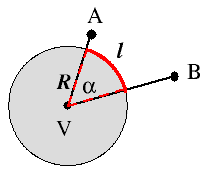
A plane angle, α, is made up of the lines that from two points A and B meet at a vertex V: it is defined by the arc length (red curve in the figure on the left) of a circle subtended by the lines and by the radius R of that circle (dotted red lines),[8A. V. Arecchi, T. Messadi, and R. J. Koshel
“Field Guide to Illumination”
SPIE Press, Bellingham, WA, 2007, p. 2., L4"Solid Angle". Optipedia: SPIE Press books opened for your reference.
Excerpt from "Field Guide to Illumination" by Angelo V. Arecchi, Tahar Messadi, R. John Koshel.] as shown on the left. The dimensionless unit of plane angle is the radian. The value in radians of a plane angle α is the ratio

α = ℓ R

of the length ℓ of a circular arc to its radius R. It follows that the plane angle subtended by the full circle measures 2π radians.

Si definisce angolo solido ciascuna delle due regioni in cui viene suddiviso lo spazio dalla superficie formata dalle semirette passanti per uno stesso punto (detto vertice dell'angolo solido) e per i punti di una curva chiusa semplice tracciata su una superficie non contenente il vertice. L'unità di misura dell'angolo solido Ω è lo steradiante. La misura in steradianti dell'angolo solido Ω è definita dal rapporto Ω = A/R² tra l'area A della porzione di superficie sferica di raggio R vista sotto l'angolo Ω e il quadrato del raggio, ed è indipendente dal particolare valore del raggio scelto. L'angolo solido sotteso da una superficie generica rispetto a un punto P è dunque equivalente a quello sotteso dalla proiezione della stessa superficie su una sfera di raggio qualsiasi centrata in P. Dalla precedente definizione consegue che l'angolo solido sotteso dall'intera superficie sferica misura 4π. Per avere la misura in gradi quadrati si moltiplica il valore in steradianti per (180/π)², ovvero per 3282,8 (circa). Quindi tutta la sfera corrisponde a circa 41253 gradi quadrati.
A solid angle is made up from all the lines that from a closed curve meet at a vertex: it is defined by the surface area A of a sphere subtended by the lines and by the radius R of that sphere,[8A. V. Arecchi, T. Messadi, and R. J. Koshel
“Field Guide to Illumination”
SPIE Press, Bellingham, WA, 2007, p. 2., L4"Solid Angle". Optipedia: SPIE Press books opened for your reference.
Excerpt from "Field Guide to Illumination" by Angelo V. Arecchi,Tahar Messadi, R. John Koshel.] as shown in the Figure on the right. The dimensionless unit of solid angle is the steradian. The measure in steradians of a solid angle Ω is the area A on the surface of a sphere of radius R divided by the radius squared,

Ω = A R² ,

and is independent of the particular value of the chosen radius. Because the area A of the entire spherical surface is 4πr², the definition implies that a sphere subtends 4π steradians at its center. By the same argument, the maximum solid angle that can be subtended at any point is 4π steradians.
Concisely, the solid angle Ω subtended by a surface S is defined as the surface area Ω of a unit sphere covered by the surface’s projection onto the sphere.[L5(a) Weisstein, E. W. "Solid Angle,"
From MathWorld - A Wolfram Web Resource.
(b) Wikipedia contributors, "Solid angle,"
Wikipedia, The Free Encyclopedia.] href="#L4">L4Weisstein, E. W. "Solid Angle,"
From MathWorld - A Wolfram Web Resource.] That’s a very complicated way of saying the following: You take a surface, like the bright red circle in the figure on the right. Then you project the edge of the circle (but in general it could be any closed curve) to the center of a sphere of any radius R. The projection intersects the sphere and forms a surface area A. Then you calculate the surface area of your projection and divide the result by the radius squared. That's it.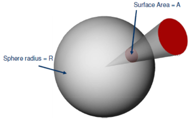

The infinitesimal element of a solid angle Ω is given by dΩ = dA R² , where dA is the surface area element in spherical coordinates defined in [N3Surface area element in spherical coordinates.], so that

dΩ = sinθ dθ dφ

is equal to the differential surface area on the unit sphere. Its integral over the solid angle of all space being subtended is the surface area of the unit sphere, which is 4 π steradians.[L5(a) Weisstein, E. W. "Solid Angle,"
From MathWorld - A Wolfram Web Resource.
(b) Wikipedia contributors, "Solid angle,"
Wikipedia, The Free Encyclopedia.]

Ω = ∫ Ω dΩ = π ∫ 0 sinθ dθ 2π ∫ 0 dφ = [−cosθ ]^{^{^π}}₀ ⋅ [φ ]^{^{^2π}}₀ = 4 π

Volume of a spherical shell of infinitesimal thickness. Consider two spheres, both centered in the origin: the inner with radius r and the outer with radius r + dr. To compute the volume of the spherical shell between their two surfaces, proceed as follows:

dV	= 4 / 3 π (r + dr)³ − 4 / 3 π r³
	= 4 / 3 π (r³ + 3r²dr + 3r dr² + dr³ − r³	(N5.1)
	= 4 / 3 π (3r²dr + 3r dr² + dr³)
	≈ 4 π r²dr

where, in the last equality, the terms drⁿ with n > 1 have been neglected. In a different way, using differentiation of volume V = 4 3 π r³ w.r.t. radius, you get area (rate of change of volume is area)

d V d r = 4 π r² ⇒ d V = 4 π r² d r

(N5.2)

Links

(a) Wikipedia contributors, "Spherical harmonics." Wikipedia, The Free Encyclopedia.
https://en.wikipedia.org/wiki/Spherical_harmonics (accessed October 3, 2018).
(b) Citizendium contributors, "Spherical harmonics." Citizendium, The Citizens' Compendium.
http://en.citizendium.org/wiki/Spherical_harmonics (accessed January 23, 2019).
(c) Weisstein, Eric W. “Spherical Harmonic.” From MathWorld − A Wolfram Web Resource.
http://mathworld.wolfram.com/SphericalHarmonic.html (accessed October 3, 2018).
Wikipedia contributors, "Table of spherical harmonics." Wikipedia, The Free Encyclopedia.
https://en.wikipedia.org/wiki/Table_of_spherical_harmonics (accessed October 3, 2018).
Mark E. Tuckerman, “The Schrödinger equation for the hydrogen atom and hydrogen-like cations”, 2011-10-26.
(Lecture 8: CHEM-UA 127: Advanced General Chemistry I)
http://www.nyu.edu/classes/tuckerman/adv.chem/lectures/lecture_8/node5.html (accessed October 31, 2018).
“Solid Angle”. Optipedia: SPIE Press books opened for your reference. Excerpt from “Field Guide to Illumination” by Angelo V. Arecchi, Tahar Messadi, R. John Koshel.[4A. V. Arecchi, T. Messadi, and R. J. Koshel
“Field Guide to Illumination”
SPIE Press, Bellingham, WA, 2007, p. 2.]
http://spie.org/publications/fg11_p02_solid_angle (accessed November 12, 2018).
(a) Weisstein, Eric W. “Solid Angle.” From MathWorld − A Wolfram Web Resource.
http://mathworld.wolfram.com/SolidAngle.html (accessed October 4, 2018).
(a) Wikipedia contributors, “Solid angle.” Wikipedia, The Free Encyclopedia.
https://en.wikipedia.org/wiki/Solid_angle (accessed October 4, 2018).
Citizendium contributors, “Hydrogen-like atom”; Citizendium, The Citizens' Compendium.
http://en.citizendium.org/wiki/Hydrogen-like_atom (unapproved; accessed December 17, 2018).