Charge Distributions.

1. Discrete Charge Distributions
2. Continuous Charge Distributions
3. Distribution of charges in atoms and molecules
4. The Probability Density Function of a Distribution of Charges: definitions and properties
   1. Joint and Marginal Probability Density Function
   2. Cumulative Distribution Function (CDF)
   3. Derivatives
   4. Taylor Series Expansion
   5. Moments and Moment Generating Function (MGF)
   6. Characteristic Function
   7. Transformation of the Random Vector Variable
5. Electrostatics
Unit Converter
6. References
7. Notes
8. Links

1. - Discrete Charge Distributions

A point charge is a point particle[N1A point particle defines a particle which lacks spatial extension.] which has an electric charge. There are two types of electric charges: positive and negative. The elementary charge, a fundamental physical constant usually denoted as e, is the electric charge carried by a single proton, whereas a single electron has charge −e. In the International System of Units (SI) the elementary charge has a measured value of approximately 1.602 176 6208(98)×10⁻¹⁹ C.[1(a) Mohr, P. J.; Newell, D. B.; Taylor, B. N.
Reviews of Modern Physics 2016, 88, 035009, 73 pages.
(b) Mohr, P. J.; Newell, D. B.; Taylor, B. N.
J. Phys. Chem. Ref. Data 2016, 45, 043102, 74 pages.] In the natural system of Hartree atomic units (usually abbreviated “au” or “a.u.”)[N2Definition of Hartree atomic units.] the elementary charge functions as the unit of electric charge, that is e is equal to 1.

All observable charges occur in integral amounts of the fundamental unit of charge e, that is, charge is quantized. Any observable charge occurring in nature can be written Q = ±Ne, where N is an integer.[2Tipler, Paul A.; Mosca, Gene
"Physics for Scientists and Engineers", - 5th ed.
W. H. Freeman and Company, San Francisco, 2004; Vol. I, p. 653.]

The amount of electric charge per unit volume is given by the charge density, ρ(r), whose SI units are C⋅m⁻³. The atomic unit of charge density (e/a₀³, where a₀ = 0.529 177 210 67(12) × 10⁻¹⁰ m is the radius of the first Bohr orbit for hydrogen) is equal to 1.081 202 3770(67) × 10¹² C ⋅ m⁻³.[1(a) Mohr, P. J.; Newell, D. B.; Taylor, B. N.
Reviews of Modern Physics 2016, 88, 035009, 73 pages.
(b) Mohr, P. J.; Newell, D. B.; Taylor, B. N.
J. Phys. Chem. Ref. Data 2016, 45, 043102, 74 pages.]

For an ensemble of N point charges q_i located at points R_i (i = 1, 2, …, N), the total charge Q is the sum of the N individual point charges:

Q = N ∑ i=1 qi

(1.1)

and the total charge density is the sum of the N individual charge densities

ρ(r) = N ∑ i=1 qi δ(r − Ri)

(1.2)

which are expressed in terms of the Dirac “delta” functions, δ(r − R_i).[3Dirac, P. “The Principles of Quantum Mechanics”
Oxford at the Clarendon Press: 1958., 4Messiah, A. “Quantum Mechanics”, Volume I
North-Holland Publishing Company, Amsterdam: 1970, pp. 179-184 and 468-471., N3Three-Dimensional Dirac Delta Function.]  The function  δ(r − R_i)  is equal to zero everywhere but at the single point  r = R_i,  where it is singular in such a manner that

∫ δ(r − Ri) d3r = 1

(1.3)

Integrating eq. (1.2) over any volume that contains all the R_i yields, because of eq. (1.3), the total charge of the distribution, i.e. Eq (1.1)

Q = ∫ ρ(r) d3r = N ∑ i=1 qi ∞ ∫ −∞ δ(r − Ri) d3r = N ∑ i=1 qi

Strictly speaking, it would not be possible to define a density function for a discrete distribution of charges, since the density is intrinsically a continuous function. The use of the Dirac “delta” function allows defining a generalized density function that substantially unifies the treatment of discrete and continuous distributions. This means, for instance, that formulas given for a continuous distribution of charges can be used as well for discrete distributions.

TEXT TO BE MOVED SOMEWHERE ELSE

The sum of the vectors q_i R_i defines the dipole moment vector of the distribution

p = N ∑ i=1 qi Ri

(1.7)

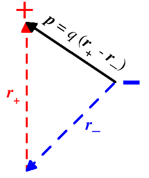
In particular, an ensemble of two point-like particles carrying charges of the same strength q and opposite sign represents an electric dipole. An electric dipole can be characterized by its electric dipole moment, a vector quantity that points from the negative charge (q₁ = −q at location r₁ = r₋) towards the positive charge (q₂ = +q at location r₂ = r₊), so that it is defined by the difference

p = q (r+ − r−)

(1.8)

The magnitude of the electric dipole moment is given by the value of the charge q times the distance of the opposite charges. It is a measure of the polarity of the charge distribution, that is of the degree of local charge separation. In other words, a dipole exists when the centers of positive and negative charge distribution do not coincide. Though the position vectors r₊ and r₋ are defined with respect to some reference system of coordinates, it is clear from eq. (1.8) that the electric dipole moment of a pair of opposite charges does not depend on the choice of origin. This fact holds also in the general case of eq. (1.7), provided the overall charge of the system is zero. Indeed, if all the position vectors, r_i, are moved to a new origin r₀ (i.e. r_i → r_i − r₀), then eq. (1.7) becomes:

p(r0) = N ∑ i=1 qi (ri − r0) = N ∑ i=1 qi ri − Q r0

(1.9)

which is independent of r₀ only if Q = 0.[N?4Conventional choice of the origin for charged systems.]

The SI units for electric dipole moment are coulomb-meter (C⋅m), however the most commonly used unit is the debye (D), which is a CGS unit. A debye is 10⁻¹⁸ esu⋅cm and about 3.336 × 10⁻³⁰ C⋅m. An atomic unit of electric dipole moment is e⋅a₀ and is about 8.478 × 10⁻²⁹ C⋅m.

A general distribution of electric point-charges may be characterized, in addition to its net charge and its dipole moment, by its electric quadrupole moment and, eventually, by higher order moments. The electric quadrupole moment is a symmetric rank-two tensor (i.e. a 3×3 matrix with 9 components, but because of symmetry only 6 of these are independent).

Θ = N ∑ i=1 qi ri ri† = N ∑ i=1 qi xixi xiyi xizi yixi yiyi yizi zixi ziyi zizi

(1.10)

As with any multipole moment, if a lower-order moment (monopole or dipole in this case) is non-zero, then the value of the quadrupole moment depends on the choice of the coordinate origin. If all the position vectors, r_i in eq. (1.10), are moved to a new origin r₀ (i.e. r_i → ri − r0), eq. (1.10) becomes:</sub>

Θ(r0) = N ∑ i=1 qi (ri − r0) (ri − r0)† = N ∑ i=1 qi ri ri† − p r0† − r0 p† + Q r0 r0†

(1.11)

which states that Θ is independent of r₀ (i.e. does not depend on the choice of origin) only if p = 0 and Q = 0. For example, the quadrupole moment of an ensemble of four same-strength point-charges, arranged in a square with alternating signs, is coordinate independent.

The SI units for electric quadrupole moment are C⋅m², however the most commonly used unit is the buckingham (B), which is a CGS units. A buckingham is 1 × 10⁻²⁶ statC⋅cm² and is equivalent to 1 D⋅Å. An atomic unit of electric quadrupole moment is e⋅a0² and is about 4.486 551 484(28) × 10⁻⁴⁰ C⋅m².

2. - Continuous Charge Distributions

“Often it is convenient to ignore the fact that charges come in packages like electrons and protons, and think of them as being spread out in a continuous smear − or in a 'distribution,' as it is called. This is O.K. so long as we are not interested in what is happening on too small a scale. We describe a charge distribution by the 'charge density,' ρ(r) ≡ ρ(x,y,z). If the amount of charge in a small volume ΔV₁ located at the point r₁ is Δq₁, then ρ is defined by”[L1“Coulomb’s law; superposition”
The Feynman Lectures on Physics, Online Edition,
Volume II, Chapter 4, Section 4.2]

Δq1 = ρ(r1) ΔV1

(2.1)

As always, the volume integral of the charge density ρ(r) over a region of space V in ℝ³ is the charge contained in that region.

q =   ∫ V ρ(r) d3r =   ∫ V ρ(r) dV =   ∭ V ρ(x,y,z) dx dy dz

(2.2)

In the Euclidean space, the components of the position vector r are the cartesian coordinates x, y and z, and the volume element dV is given by the product of the differentials of the cartesian coordinates, dV = dx dy dz.

3. - Distribution of charges in atoms and molecules.

Matter consists of atoms that are electrically neutral. Each atom has a tiny but massive nucleus that contains protons and neutrons. Protons are positively charged, whereas neutrons are uncharged. The number of protons in the nucleus is the atomic number Z of the element. Surrounding the nucleus is an equal number of negatively charged electrons, leaving the atom with zero net charge. The electron is about 2000 times less massive than the proton, yet the charges of these two particles are exactly equal in magnitude.[2Tipler, Paul A.; Mosca, Gene
"Physics for Scientists and Engineers", - 5th ed.
W. H. Freeman and Company, San Francisco, 2004; Vol. I, p. 653.]

The Heisenberg's uncertainty principle states that the more precisely the position of an electron is determined, the less precisely its momentum can be known, and vice versa.[5Heisenberg, W. Zeitschrift für Physik 1927, 43, 172–198., 6Sen, D. Current Science 2014, 107, 203-218.] Therefore, we can not say exactly where the electron is, but quantum mechanics provides a recipe for calculating the probability ρ(x,y,z) dx dy dz that it is in an element of volume dV = dx dy dz at a particular point in the coordinate space x, y, z, and this quantity is expressed in terms of a function ρ(x,y,z) called “electron probability density” or simply “electron density”. This does not imply that the electron is “diluted” throughout the region of space in which the electronic density is non-zero: in a certain volume dV there may be a very small probability of finding the electron; but if you find it there, you find it all. However, in many cases (for example, dispersion of X-rays, forces on atoms), a system consisting of a large number of electrons behaves exactly as if the electrons were distributed nonuniformly over a region of space, so that each point in space is characterized by a certain fraction of charge or partial charge, which is identical to the electron probability density. In fact, for large numbers, the frequency tends to probability. Therefore, a map showing how the electron probability density varies from point to point in a molecule, i.e. a map of the cumulative distribution of the charge of all the electrons of the molecule, is a model of the electronic structure of the molecule.[7Shusterman, G. P.; Shusterman, A. J.
J. Chem. Ed. 1997, 74, 771-776.]

Two or more atoms held together by chemical bonds give an electrically neutral entity called molecule.[8IUPAC. Compendium of Chemical Terminology, 2nd ed. (the "Gold Book").] Since atomic nuclei are much heavier than electrons (about 2000 times), they move more slowly. Hence, to a good approximation (the Born-Oppenheimer approximation[9Born, M.; Oppenheimer, R. Annalen der Physik 1927, 389, 457-484.]), we can consider that the electrons are moving in a field of fixed nuclei.

The molecular charge density ρ_molecule(r,{R_i}) is the sum of the nuclear density ρ_nuclei(r,{R_i}) and the electron density ρ_electrons(r,{R_i}):

ρmolecule(r,{Ri}) = ρnuclei(r,{Ri}) − ρelectrons(r,{Ri})

(3.1)

where the variable r is the position vector and the nuclear coordinates {R_i} are fixed parameters. The − sign accounts for the negative charge of the electrons.

The nuclei in a molecule are a discrete distribution of positive charges {Z_i} at fixed positions {R_i} so that their density has the following expression:

ρnuclei(r,{Ri}) = N ∑ i=1 Zi δ(r − Ri)

(3.2)

according to eq. (1.2). The charge of each nucleus is given by its atomic number Z_i. The expression of the electron density, a continous probability distribution, depends on the quantum-mechanical recipe used for its calculation or by the functional model used to analyze experimental x-ray diffraction data. Eventually, it can be known as a set of numerical values defined over a grid of data points {r_j}.

Any molecular probability charge distribution involves both a continuous and a discrete part (eq. 3.1). As noted previously, the use of the generalized probability density function (eq. 3.2) substantially unifies the treatment of continuous and discrete distributions.

4. - The Probability Density Function (PDF) of a Distribution of Charges: definitions and properties

4.1. - Joint and Marginal Probability Density Function.   In the previous section, the electron probability density has been introduced as the scalar-valued function ρ(x,y,z) of the three Cartesian coordinates x, y, z in the Euclidean space ℝ³ such that, multiplied by an infinitesimal element of volume dV = dx dy dz at point (x,y,z), gives the probability of finding the electron at that point. This definition can be extended to any charge distribution.

More correctly, the function ρ(x,y,z) should be called a joint probability density function, where the word “joint” stresses the fact that this probability is linked to the occurrence of a triple of values, one for each of the three variables x, y, z. In common practice, it is simply called probability density function (PDF), or even more shortly, probability function or density function.

The PDF has the following properties:

1.  ρ(x,y,z) ≥ 0,
2. ∞ ∫ −∞ ∞ ∫ −∞ ∞ ∫ −∞ ρ(x,y,z) dx dy dz = 1.
   Of course, this normalization property is valid for a single point charge. In words, it says that the probability of finding a point-like charge everywhere in ℝ³ is equal to one. For any distribution of charges, the total PDF is the sum of the PDFs of all the elementary charges, and its integral over ℝ³ gives the total charge of the distribution, according to eq. (2.2).

A number of marginal PDF's can be obtained from the joint PDF ρ(x,y,z) by means of the following definitions:

ρ(x) = ∞ ∫ −∞ ∞ ∫ −∞ ρ(x,y,z) dy dz	(4.1.1)
ρ(y) = ∞ ∫ −∞ ∞ ∫ −∞ ρ(x,y,z) dx dz	(4.1.2)
ρ(z) = ∞ ∫ −∞ ∞ ∫ −∞ ρ(x,y,z) dx dy	(4.1.3)
ρ(x,y) = ∞ ∫ −∞ ρ(x,y,z) dz	(4.1.4)
ρ(x,z) = ∞ ∫ −∞ ρ(x,y,z) dy	(4.1.5)
ρ(y,z) = ∞ ∫ −∞ ρ(x,y,z) dx	(4.1.6)

Therefore, the PDF associated with each variable x, y, and z alone (or with any pair of variables xy, xz, and yz) is called marginal density function, and can be deduced from the joint probability density associated with the variables x,y,z by integrating over all values of the remaining two (or one) variables.
The radial density function is the most important example of marginal PDF that we will find in this manual.

It proves useful to analyse the PDF with the aid of related functions which point out features and properties of the PDF itself. A few of them will be considered in the following.

4.2. - Cumulative Distribution Function (CDF). The (joint) cumulative distribution function D(x,y,z) is defined as the probability to find some charge within the semi-infinite parallelepiped with upper limits defined by x, y, z. It can be expressed as the integral of its (joint) probability density function ρ(x,y,z) as follows:

D(x,y,z) = x ∫ −∞ y ∫ −∞ z ∫ −∞ ρ(x',y',z') dx' dy' dz'

(4.2.1)

The (joint) cumulative distribution function D(x,y,z) has the following properties:

1. it is right-continuous in each of its variables,
2. it is monotonically increasing for each of its variables,
3. it tends to 0 as any of its variables tends to minus infinity.
4. it tends to 1 as all its variables tend to positive infinity, As noted previously, this normalization property is valid for a single point charge. For any distribution of charges, the total CDF is the sum of the CDFs of all the elementary charges, and its integral over ℝ³ gives the total charge of the distribution,

Of course, a CDF exists for all the marginal PDFs of ρ(x,y,z), i.e.:

D(x,y) = x ∫ −∞ dx' y ∫ −∞ dy' ∞ ∫ −∞ ρ(x',y',z') dz' = x ∫ −∞ y ∫ −∞ ρ(x',y') dx' dy'	(4.2.2)
D(x,z) = x ∫ −∞ dx' z ∫ −∞ dz' ∞ ∫ −∞ ρ(x',y',z') dy' = x ∫ −∞ z ∫ −∞ ρ(x',z') dx' dz'	(4.2.3)
D(y,z) = y ∫ −∞ dy' z ∫ −∞ dz' ∞ ∫ −∞ ρ(x',y',z') dx' = y ∫ −∞ z ∫ −∞ ρ(y',z') dy' dz'	(4.2.4)
D(x) = x ∫ −∞ dx' ∞ ∫ −∞ ∞ ∫ −∞ ρ(x',y',z') dy' dz' = x ∫ −∞ ρ(x') dx'	(4.2.5)
D(y) = y ∫ −∞ dy' ∞ ∫ −∞ ∞ ∫ −∞ ρ(x',y',z') dx' dz' = y ∫ −∞ ρ(y') dy'	(4.2.6)
D(z) = z ∫ −∞ dz' ∞ ∫ −∞ ∞ ∫ −∞ ρ(x',y',z') dx' dy' = z ∫ −∞ ρ(z') dz'	(4.2.7)

In turn, the PDFs can be obtained as the derivative of their CDF:

ρ(x) = dD(x) / dx	(4.2.8)
ρ(y) = dD(y) / dy	(4.2.9)
ρ(z) = dD(z) / dz	(4.2.10)
ρ(x,y) = ∂2D(x,y) / ∂x ∂y	(4.2.11)
ρ(x,z) = ∂2D(x,z) / ∂x ∂z	(4.2.12)
ρ(y,z) = ∂2D(y,z) / ∂y ∂z	(4.2.13)
ρ(x,y,z) = ∂3D(x,y,z) / ∂x ∂y ∂z	(4.2.14)

In their 1968 study of the four lowest ¹Σ⁺ states of the LiH molecule, Brown and Shull used the cumulative distribution function D(z) of Eq. (4.2.7) and the marginal probability density function ρ(z) of Eq. (4.2.10) to analyse the calculated wave functions.[10Brown, Richard E.; Shull, Harrison
Int. J. Quantum Chem. 1968, 2, 663-685.] These two functions were designated respectively electron count and planar density. Since the Li and H nuclei are situated on the z-axis with the axis origin at the molecular midpoint, the electron count function D(z) simply denotes the number of electrons on the negative side of the xy-plane intersecting the z-axis at the point z, and the planar density ρ(z) = D'(z) is the density of electrons in this plane.[10Brown, Richard E.; Shull, Harrison
Int. J. Quantum Chem. 1968, 2, 663-685.]  In 1970, Politzer and Harris used the electron count function D(z) to propose a definition of the charge on an atom in linear molecules.[11Politzer, Peter; Harris, Roger R.
J. Am. Chem. Soc. 1970, 92, 6451-6454.]

In 1979 Streitwieser and coworkers suggested to use the bivariate marginal density ρ(x,z) of Eq. (4.5) or (4.2.12), called the electron projection function, for aiding visualization of the electron density. Projecting the electron density function ρ(x,y,z) into the xz-plane corresponds to summing ρ(x,y_i,z) over all  y_i = constant  parallel planes. Hence, there is no arbitrariness about the choice of one of these planes in which to display the PDF. Because it compresses the total electron density onto a two-dimensional grid, it is ideal for graphical representation and simplifies qualitative electron density analyses.[12(a)  Streitwieser, A. Jr.; Collins, J. B.; McKelvey, J. M.; Grier, D.; Sender, J.; Toczko, A. G.
Proc. Nati. Acad. Sci. USA 1979, 76, 2499-2502.
(b)  Collins, J. B.; Streitwieser, A. Jr.  J. Comput. Chem. 1980, 1, 81-87.
(c)  Bachrach, S. M.; Streitwieser, A.  J. Comput. Chem. 1989, 10, 514-519.
(d)  Agrafiotis, D. K.; Tansy, B.; Streitwieser, A.  J. Comput. Chem. 1990, 11, 1101-1110.]  The electron projection function was also proposed as a generalization for planar or nearly planar systems of the partitioning of space introduced by Politzer[11Politzer, P.; Harris, R. R.
J. Am. Chem. Soc. 1970, 92, 6451-6454.] for linear molecules. However the projection method gives integrated charges that have no fundamental significance and which are at best only approximations to charges that correspond to zero-flux surfaces.[13Glaser, R. J. Comput. Chem. 1989, 10, 118-135.]

4.3. - Derivatives.  The density function ρ(x,y,z) = ρ(r) is a continuous function which operates on a vector variable r = (x, y, z)^† ∈ ℝ³ and returns a scalar, i.e. ρ(r): ℝ³ → ℝ.  Since ρ(r) assigns a scalar value to any point r in space, it defines a scalar field.  The function can be differentiated to any order with respect to each of the variables x, y, and z, the other variables being understood to be held constant during the differentiation. Such derivatives are known as partial derivatives. The first-order partial derivatives are

∂ ρ / ∂ x = ρx,      ∂ ρ / ∂ y = ρy,      ∂ ρ / ∂ z = ρz

(4.3.1)

As the variables x, y, z are the components of the (column) vector r, similarly ∂ / ∂ x , ∂ / ∂ y , ∂ / ∂ z are the components of the gradient vector operator, “grad”, more commonly indicated by the symbol ∇, denominated “nabla” or “del”.[N4The vector differential operator ∇.] So, the three scalar expressions of Eq (4.3.1) are equivalent to the vector expression

grad ρ = ∇ ρ = ∂ ρ(r) / ∂ r = ∂ / ∂ x ∂ / ∂ y ∂ / ∂ z ρ = ρx ρy ρz

(4.3.2)

The gradient of ρ(r) is a mapping which operates on a continuous scalar function of a vector variable and returns a continuous vector-valued function, i.e. ∇ ρ(r): ℝ³ → ℝ³.  It is a physical quantity that has both magnitude and direction.  Since it assigns a vector to any point r in space, it defines a vector field.  Its components are organized in a column, so that it is referred to as a column vector or column matrix, i.e. a matrix which has only one column. The transpose of a column matrix is another matrix which has only one row and is called a row matrix or row vector.[N5Definition of column matrix and column vector]

By differentiating the three first-order partial derivatives of Eq. (4.3.1) with respect to x, y, and z, three second-order partial derivatives are obtained

∂2 ρ / ∂ x2 = ∂ ρ / ∂ x ( ∂ ρ / ∂ x ) = ρxx,      ∂2 ρ / ∂ y2 = ∂ ρ / ∂ y ( ∂ ρ / ∂ y ) = ρyy,      ∂2 ρ / ∂ z2 = ∂ ρ / ∂ z ( ∂ ρ / ∂ z ) = ρzz

(4.3.3)

together with six second-order mixed derivatives

ρxy = ∂2 ρ / ∂ x ∂ y = ∂ ρ / ∂ x ( ∂ ρ / ∂ y ) = ∂ ρ / ∂ y ( ∂ ρ / ∂ x ) = ∂2 ρ / ∂ y ∂ x = ρyx,
ρxz = ∂2 ρ / ∂ x ∂ z = ∂ ρ / ∂ x ( ∂ ρ / ∂ z ) = ∂ ρ / ∂ z ( ∂ ρ / ∂ x ) = ∂2 ρ / ∂ z ∂ x = ρzx,	(4.3.4)
ρyz = ∂2 ρ / ∂ y ∂ z = ∂ ρ / ∂ y ( ∂ ρ / ∂ z ) = ∂ ρ / ∂ z ( ∂ ρ / ∂ y ) = ∂2 ρ / ∂ z ∂ y = ρzy

where it appears that the mixed derivatives (assuming that they are continuous) do not depend on the order of the differentiation.  Higher-order partial and mixed derivatives are again defined recursively, e.g.

∂i+j+k ρ / ∂xi ∂yj ∂zk = ρ(i,j,k)

(4.3.5)

The second order partial and mixed derivatives of Eqs (4.3.3) and (4.3.4) are found in the result of applying the “nabla” operator twice in sequence. How they are structured in the result depends on how the “nabla” operator is applied. Since ∇ can be viewed as a 3×1 matrix,[N5Definition of column matrix and column vector] let's take the Kronecker product[14Zhang, H.; Ding, F.
Journal of Applied Mathematics 2013, Article ID 296185, 8 pages., N6Kronecker product (definition), L4Wikipedia contributors, "Kronecker product,"
Wikipedia, The Free Encyclopedia., L5Weisstein, E. W. "Kronecker Product."
From MathWorld - A Wolfram Web Resource.] of ∇ with its transpose ∇^†

∇⊗∇†ρ = ∂ ∇† / ∂ x ∂ ∇† / ∂ y ∂ ∇† / ∂ z ρ = ∂2 / ∂ x2 ∂2 / ∂ x ∂ y ∂2 / ∂ x ∂ z ∂2 / ∂ y ∂ x ∂2 / ∂ y2 ∂2 / ∂ y ∂ z ∂2 / ∂ z ∂ x ∂2 / ∂ z ∂ y ∂2 / ∂ z2 ρ = ρxx ρxy ρxz ρyx ρyy ρyz ρzx ρzy ρzz ≡ H(r)

(4.3.6)

If all second partial derivatives of ρ(r) exist and are continuous over the domain of the function, then the Hessian matrix H of ρ(r) is a square symmetric 3×3 matrix, defined and arranged as in Eq (4.3.6).[L6Wikipedia contributors, "Hessian matrix,"
Wikipedia, The Free Encyclopedia.]

The Kronecker product ∇^†⊗∇ = (∇⊗∇^†)^† can be calculated in a similar way, leading to the definition of the Jacobian matrix:[L7Wikipedia contributors, "Jacobian matrix and determinant,"
Wikipedia, The Free Encyclopedia., L8Weisstein, E. W. "Jacobian."
From MathWorld - A Wolfram Web Resource.]

∇†⊗∇ ρ = ∂ ∇ / ∂ x ∂ ∇ / ∂ y ∂ ∇ / ∂ z ρ = ∂ ρx / ∂ x ∂ ρx / ∂ y ∂ ρx / ∂ z ∂ ρy / ∂ x ∂ ρy / ∂ y ∂ ρy / ∂ z ∂ ρz / ∂ x ∂ ρz / ∂ y ∂ ρz / ∂ z = ρxx ρyx ρzx ρxy ρyy ρzy ρxz ρyz ρzz ≡ J(r)

(4.3.7)

The Jacobian matrix is the matrix of all first-order partial derivatives of the vector-valued function ∇ρ(r), defined and arranged as in Eq. (4.3.7). (Note that some literature defines the Jacobian as the transpose of the matrix given in Eq. (4.3.7).) It defines a linear map ℝ³ → ℝ³, which is the generalization of the usual notion of derivative, and is called the derivative or the gradient of ∇ρ at r.[L9Granados, A. "Taylor Series For Multi-Variable Functions." 2015.
A ResearchGate Web Resource.]

The Jacobian matrix of the gradient of the scalar function ρ(r) is the transpose of the Hessian matrix, and since the latter is a symmetric square matrix, they are equal. In a sense, both the gradient and Jacobian are “first derivatives”: the former the first derivative of a scalar function of r, the latter the first derivative of a vector function of r. The Hessian matrix in a sense is the “second derivative” of a scalar function of r.

H[ρ(r)] = J[∇ρ(r)]†

(4.3.8)

The Kronecker product ∇⊗∇ supplies the same derivatives of the Jacobian matrix in Eq. (4.3.7), but organized in a single 9×1 column matrix:

∇⊗∇ ρ = ∂ ∇ / ∂ x ∂ ∇ / ∂ y ∂ ∇ / ∂ z ρ = ∂ ρx / ∂ x ∂ ρy / ∂ x ∂ ρz / ∂ x ∂ ρx / ∂ y ∂ ρy / ∂ y ∂ ρz / ∂ y ∂ ρx / ∂ z ∂ ρy / ∂ z ∂ ρz / ∂ z ≡ vec J(r)

(4.3.9)

where the “vec” (vectorizaton) operator has been introduced.[15Magnus, J. R.; Neudecker, H.
The Annals of Statistics 1979, 7, 381-394., 16Henderson, H. V.; Searle, S. R.
Linear and Multilinear Algebra 1981, 9, 271-288., L10Wikipedia contributors, "Vectorization_(mathematics),"
Wikipedia, The Free Encyclopedia.]

It is worth noting that the same result of Eq. (4.3.6) can be obtained by multiplying ∇ and ∇^† according to the usual matrix multiplication rule, provided that ∇ is represented as a 3×1 column matrix (which makes ∇^† a 1×3 row matrix):

∇∇†ρ = ∂ / ∂ x ∂ / ∂ y ∂ / ∂ z ∂ / ∂ x ∂ / ∂ y ∂ / ∂ z ρ = ∂2 / ∂ x2 ∂2 / ∂ x ∂ y ∂2 / ∂ x ∂ z ∂2 / ∂ y ∂ x ∂2 / ∂ y2 ∂2 / ∂ y ∂ z ∂2 / ∂ z ∂ x ∂2 / ∂ z ∂ y ∂2 / ∂ z2 ρ = ρxx ρxy ρxz ρyx ρyy ρyz ρzx ρzy ρzz ≡ H(r)

(4.3.10)

i.e. ∇⊗∇^† = ∇∇^†.  At this point we have the rules to evaluate all the thirds and higher derivatives of ρ(r) at any point r = (x, y, z)^† ∈ ℝ³. For example, the derivative or the gradient of the Jacobian matrix J(r) is the 3×9 matrix of the thirds derivatives of ρ(r), defined and arranged as follows:

∇†⊗J = ∂ J / ∂ x ∂ J / ∂ y ∂ J / ∂ z = ρxxx ρxyx ρxzx ρyxx ρyyx ρyzx ρzxx ρzyx ρzzx ρxxy ρxyy ρxzy ρyxy ρyyy ρyzy ρzxy ρzyy ρzzy ρxxz ρxyz ρxzz ρyxz ρyyz ρyzz ρzxz ρzyz ρzzz

(4.3.11)

Similarly, the fourth derivatives of ρ(r) are the elements of the 3×27 matrix ∇^†⊗∇^†⊗J = ∇^⊗2J = ∇^⊗3∇ ρ(r) i.e. the fourth derivatives of ρ are the second derivatives of the Jacobian matrix and the third derivatives of the gradient of ρ.

In general, we'll use the notation of Eq. (4.3.9) to compute the derivatives of the scalar field ρ(r), so that its n-th derivatives are the components of the 3ⁿ×1 column matrix of Eq. (4.3.12):

∇⊗∇⊗ … ∇⊗ n-times ρ(r) = ∇⊗(n) ρ(r) = ∇⊗(n−1)⊗∇ ρ(r) = ∇⊗(n−2)⊗ J(r)

(4.3.12)

where sometimes the symbol ⊗ is omitted.

The dot product of the vector operator ∇ with the gradient vector of ρ(r) defines the Laplacian of ρ(r), a scalar field:

∇⋅∇ρ = ∇2ρ = Δρ = ∂2 / ∂ x2 + ∂2 / ∂ y2 + ∂2 / ∂ z2 ρ = ∂ / ∂ x ∂ / ∂ y ∂ / ∂ z ∂ / ∂ x ∂ / ∂ y ∂ / ∂ z ρ = ∇†∇ρ

(4.3.13)

It's worth noting that the Laplacian of ρ(r) is equal to the trace of the Hessian (Jacobian) matrix of ρ(r):

Δρ(r) = ∇2ρ(r) = Tr H(r) = Tr J(r)

(4.3.14)

The Laplacian can also be defined as the divergence of the gradient of ρ(r).

The directional derivative of the scalar function ρ(r) = ρ(x,y,z), differentiable at r, along a vector u = (u_x, u_y, u_z)^† is the scalar function ∇_u ρ(r) defined by the dot product of u with the gradient of ρ(r):

∇u ρ(r) = u ⋅ ∇ρ(r)

(4.3.15)

If u is a unit vector, the directional derivative ∇_u ρ(r) is independent of the magnitude of u and depends only on its direction.  Intuitively, the directional derivative of ρ at a point r represents the rate of change of ρ with respect to a change of its argument r in the direction of u.

he Laplacian Δf(p) of a function f at a point p, is (up to a factor) the rate at which the average value of f over spheres centered at p deviates from f(p) as the radius of the sphere grows.

4.4. - Taylor series expansion.  Suppose  ρ(r): ℝ³ → ℝ is of class C ^k+1 on an open convex set S  [i.e. ρ(r) is a scalar function of a vector variable r = (x, y, z)^† ∈ ℝ³, its partial derivatives exist up to the (k+1)-th order and are continuous, it is defined over a set of points such that, given any two points A, B in that set, the line AB joining them lies entirely within that set].  If a ∈ S and r = a + h ∈ S, then the Taylor expansion for ρ(r) at point r about point a is

ρ(a + h) = k ∑ j=0 h⊗j ⋅ ∇⊗j ρ(a) / j! + Ra,k(h)

(4.4.1)

where h = r − a, and formulas for the remainder R_a,k(h) can be obtained from the Lagrange or integral formulas for remainders, but this is beyond the aim of this manual.[17Stewart, James  "Calculus Early Transcendentals", 6th ed.
Thomson Brooks/Cole, USA, 2008, Section 11.10, p. 734., L14Stewart, J.
"Formulas for the Remainder Term in Taylor Series"]

To obtain Eq. (4.4.1), we start by supposing that ρ can be represented by a Kronecker power series[17Stewart, James  "Calculus Early Transcendentals", 6th ed.
Thomson Brooks/Cole, USA, 2008, Section 11.10, p. 734.]

ρ(a + h) = k ∑ j=0 cj ⋅ h⊗j =  c0  +  c1 ⋅ h  +  c2 ⋅ h⊗2  +  c3 ⋅ h⊗3  +  c4 ⋅ h⊗4  +  …  +  ck ⋅ h⊗k

(4.4.2)

Let’s try to determine what the coefficients c_j must be in terms of ρ. To begin, notice that if we put r = a in Eq. (4.4.2), then h = 0, and all terms after the first one are 0 and we get

ρ(a)  =  c0

(4.4.3)

Since ρ is of class C ^k+1, we can differentiate the series in Eq. (4.4.2) term by term:

∇ρ(a + h)  =  c1  +  2 c2 ⋅ h  +  3 c3 ⋅ h⊗2  +  4 c4 ⋅ h⊗3  +  …  +  k ck ⋅ h⊗(k−1)

(4.4.4)

and substitution of h = 0 in Eq. (4.4.4) gives

∇ρ(a)  =  c1

(4.4.5)

Now we differentiate both sides of Eq. (4.4.4) and obtain

∇⊗∇ρ(a + h)  =  ∇⊗2ρ(a + h)  =  2 c2  +  2⋅3 c3 ⋅ h  +  3⋅4 c4 ⋅ h⊗2  +  …  +  (k−1)⋅k ck ⋅ h⊗(k−2)

(4.4.6)

Again we put h = 0 in Eq. (4.4.6). The result is

∇⊗2ρ(a)  =  2 c2

(4.4.7)

Let’s apply the procedure one more time. Differentiation of the series in Eq. (4.4.6) gives

∇⊗∇⊗∇ρ(a + h)  =  ∇⊗3ρ(a + h)  =  2⋅3 c3  +  2⋅3⋅4 c4 ⋅ h  +  3⋅4⋅5 c5 ⋅ h⊗2  +  …  +  (k−2)⋅(k−1)⋅k ck ⋅ h⊗(k−3)

(4.4.8)

and substitution of h = 0 in Eq. (4.4.8) gives

∇⊗3ρ(a)  =  2⋅3 c3  =  3! c3

(4.4.9)

By now you can see the pattern. If we continue to differentiate and substitute h = 0, we obtain

∇⊗(k)ρ(a)  =  2⋅3⋅4⋅…⋅k ck  =  k! ck

(4.4.10)

Solving this equation for the k-th coefficient c_k, we get

ck  =  ∇⊗(k)ρ(a) / k!

(4.4.11)

This formula remains valid even for k = 0 if we adopt the conventions that 0! = 1 and ∇^⊗(0)ρ = ρ. Thus we have proved that if ρ has a Kronecker power series representation (expansion) at point a, as shown in Eq. (4.4.2), then its coefficients are given by Eq. (4.4.11). Substituting expression (4.4.11) for c_k back into the series (4.4.2), we see that if ρ has a Kronecker power series expansion at a, then it must be of the form given by Eq. (4.4.1).

For the special case a = 0, the Taylor series of Eq. (4.4.1) becomes

ρ(r) = k ∑ j=0 r⊗j ⋅ ∇⊗j ρ(0) / j! + R0,k(r)

(4.4.12)

This case arises frequently enough that it is given the special name Maclaurin series.

4.5. - Moments and Moment Generating Function (MGF).  The n-th rank moment of a discrete or continuous probability distribution, described by a probability density function ρ(r) is given by the volume integral

m(n) =   ∫ V ρ(r) r⊗n d3r = E[r⊗n]

(4.5.1)

where E is the expectation operator or mean.  The discussion of these quantities (that can be called “unnormalized traced Cartesian” moments about zero and are usually referred to as raw or crude moments[Weisstein, Eric W. "Raw Moment." From MathWorld--A Wolfram Web Resource. http://mathworld.wolfram.com/RawMoment.html] and unabridged moments[Applequist J. Chem Phys. 1984; 85:279–290]) is postponed to a specific page of the manual.  Here, we simply note that the zero-th rank moment of the distribution is just the electric charge defined by Eq. (2.2).

Given a discrete or continuous probability distribution, described by a probability density function ρ(r), the moment generating function (MGF) is defined by

Mr(s) = E(es†r)

(4.5.2)

for |s| finite, where r = (x, y, z)^† ∈ ℝ³,  s = (s_x, s_y, s_z)^† ∈ ℝ³,  and

E(es†r) ≡ ⟨es†r⟩ =   ∫ ℝ3 es†r ρ(r) d3r

(4.5.3)

is the expectation value of the function e^s†r in the variable r. Note that M_r(−s) is the two-sided (doubly infinite) Laplace transform of ρ(r),  ℒ_r[ρ(r)](s).

As its name implies, the moment generating function can be used to compute the moments of ρ(r): the kth moment about 0 is the kth derivative of the moment generating function, evaluated at s = 0. Let k_x, k_y, k_z be nonnegative integers and k = k_x + k_y + k_z. Then

∂k / ∂sxkx ∂syky ∂szkz Mr(s)	=  ∂k / ∂sxkx ∂syky ∂szkz E(es†r)
	=  E ( ∂k / ∂sxkx ∂syky ∂szkz esxx + syy + szz )
	=  E(xkx yky zkz  es†r)

Setting s = 0 = (0, 0, 0)^†, we get

∂k / ∂sxkx ∂syky ∂szkz Mr(s)|s=0 = E(xkx yky zkz)

(4.5.4)

An intuitively attractive expression for the function M_r(s), which accounts for the name “moment generating function”, can be obtained by expanding the function e^s†r = e^s⋅r as a Taylor series:

Mr(s) = E[es⋅r] = E [ ∞ ∑ j=1 s⊗j ⋅ r⊗j / j! ] = ∞ ∑ j=1 E[s⊗j ⋅ r⊗j] / j! = ∞ ∑ j=1 s⊗j / j! ⋅ E[r⊗j] = ∞ ∑ j=1 s⊗j / j! ⋅ m(j)

(4.5.5)

So, if M_r(s) exists in a neighbourhood of 0, then the k-th derivative of M_r(s) evaluated at s = 0 gives the k-th moment m^(k) of the distribution:

m(k) = E[r⊗k] = ∇⊗k Mr(s)|s=0

(4.5.6)

which is the equivalent of Eq. (4.5.4) in tensor notation.

4.6. - Characteristic function.  The characteristic function of the random vector r = (x, y, z)^† ∈ ℝ³, which has a probability density function ρ(r), is defined as the expectation value of e^is⋅r, where i = √−1 is the imaginary unit, and s = (s_x, s_y, s_z)^† ∈ ℝ³ is the argument of the characteristic function  φ_r: ℝ³ → ℂ,

φr(s)	=  E[eis⋅r]  =    ∫ ℝ3 eis⋅r ρ(r) d3r	(4.6.1)
	=  E[cos(s⋅r) + i sin(s⋅r)]
	=  E[cos(s⋅r)] + i E[sin(s⋅r)]

where the last equality in the first line is the Fourier transform of the probability density function ρ(r) with sign reversal in the complex exponential.  Observe that φ_r(s) exists for any s ∈ ℝ³ because the expectation values appearing in the last line are well-defined, as both the sine and the cosine are bounded (they take values in the interval [−1,1]). So e^is⋅r lies on the unit circle in the complex plane, so that |e^is⋅r| = 1 and giving that |φ_r(s)| ≤ 1 for all s ∈ ℝ³.  Instead, the finiteness of the moment generating function of Eq. (4.5.2) is questionable since the exponential function is unbounded, so that e^s⋅r may be very large indeed.

The characteristic function and the probability density function are each a Fourier transform of the other. So, if the characteristic function is known, the inversion theorem allows to calculate the probability density function:

ρ(r) = 1 / 2 π   ∫ ℝ3 e−is⋅r φr(s) d3s

(4.6.2)

By expanding the function e^is⋅r as a Taylor series, the characteristic function can be written in the form

φr(s) = E[eis⋅r] = E [ ∞ ∑ j=1 i j s⊗j ⋅ r⊗j / j! ] = ∞ ∑ j=1 i j E[s⊗j ⋅ r⊗j] / j! = ∞ ∑ j=1 i j s⊗j / j! ⋅ E[r⊗j] = ∞ ∑ j=1 i j s⊗j / j! ⋅ m(j)

(4.6.3)

The characteristic function can be used to find moments of the random vector r. Provided that the k-th moment exists, the characteristic function can be differentiated k times, yielding

∇⊗k φr(s) |s=0  =  ik E[r⊗k]  =  ik m(k)

(4.6.4)

4.7. - Transformation of the Random Vector Variable.  Suppose we are given a random vector variable r ∈ ℝ³ with probability density ρ(r). If u ∈ ℝ³ is a random vector variable, we define a vector-valued function f: ℝ³ → ℝ³  which takes as input the vector u and produces as output the vector r. In other words, if r₁ = x, r₂ = y, r₃ = z are Cartesian coordinates, and u₁, u₂, u₃ are some other coordinates, then the functions f₁, f₂, and f₃ establish a one-to-one correspondence between the coordinate systems: they have to be continuous, have continuous partial derivatives and single valued inverse, i.e.

r = f(u)        or        x  y  z  = f1 (u1, u2, u3) f2 (u1, u2, u3) f3 (u1, u2, u3)

(4.7.1)

Eq. (4.7.1) defines the so-called u-substitution.

Differentiating the vector  r = (x, y, z)^† = (f₁, f₁, f₁)^† = f  yields the vector  dr = (dx, dy, dz)^† = (df₁, df₂, df₃)^† = df,  which can be written more explicitly and with matrix notation as

dx  dy  dz  = d f1 (u1, u2, u3) d f2 (u1, u2, u3) d f3 (u1, u2, u3) = ∂f1 / ∂u1 du1 + ∂f1 / ∂u2 du2 + ∂f1 / ∂u3 du3 ∂f2 / ∂u1 du1 + ∂f2 / ∂u2 du2 + ∂f2 / ∂u3 du3 ∂f3 / ∂u1 du1 + ∂f3 / ∂u2 du2 + ∂f3 / ∂u3 du3 = ∂f1 / ∂u1 ∂f1 / ∂u2 ∂f1 / ∂u3 ∂f2 / ∂u1 ∂f2 / ∂u2 ∂f2 / ∂u3 ∂f3 / ∂u1 ∂f3 / ∂u2 ∂f3 / ∂u3 du1 du2 du3

(4.7.2)

or more concisely

dr = Jf(u) du

(4.7.3)

The 3×3 matrix in the last equality of Eq. (4.7.2) is the Jacobian matrix of the function f at a point u where f is differentiable. It is usually denoted by

Jf(u) = Df = ∂ (f1, f2, f3) / ∂ (u1, u2, u3) = ∂ f / ∂ u = ∇†⊗f = | ∂ f / ∂ u1   ∂ f / ∂ u2   ∂ f / ∂ u3 | = ∇† f1 ∇† f2 ∇† f3

(4.7.4)

or, component-wise: J_ij = ∂ f_i / ∂ u_j.  Notations in the second, third, and fourth members of Eq. (4.7.4) point out that the Jacobian matrix can be seen as the generalization of the usual notion of derivative, and then it is called the derivative or the differential of f at u.[L7Wikipedia contributors, "Jacobian matrix and determinant,"
Wikipedia, The Free Encyclopedia., L8Weisstein, E. W. "Jacobian."
From MathWorld - A Wolfram Web Resource.] In particular, the last three members of Eq. (4.7.4) show that the Jacobian matrix can also be thought as the gradient of f.  The vector ∂ f / ∂ u_j is the j-th column of the Jacobian matrix (it is tangent to the surface f at point u), whereas the transpose of vector ∇ f_i = grad(f_i) is the i-th row of the Jacobian matrix. As a mnemonic, it is worth noting that across a row of the Jacobian matrix the numerators are the same and down a column the denominators are the same.

Left-multiplying vectors in both members of Eq. (4.7.3) by their transpose yields the following equalities:

dr† dr = du† Jf(u)† Jf(u) du = du† g du

(4.7.5)

where the symmetric matrix g = J_f(u)^† J_f(u) is called the fundamental (or metric) tensor of the Euclidean space in curvilinear coordinates. It has elements   g_ii = | ∂ f / ∂ u_i|2  and  g_ij = ∂ f / ∂ u_i ⋅ ∂ f / ∂ u_j   for   i,j = 1, 2, 3. The matrix product  dr^† dr  in Eq. (4.7.5) is equivalent to the dot product  dr⋅dr = dr²  which is known as the first fundamental form or line element

dr2 = g11 du12 + g22 du22 + g33 du32 + 2 g12 du1 du2 + 2 g13 du1 du3 + 2 g23 du2 du3

(4.7.6)

Roughly speaking, the metric tensor g is a function which tells how to compute the distance between any two points in a given space. Its components can be viewed as multiplication factors which must be placed in front of the differential displacements du_i in the generalized Pythagorean theorem of Eq. (4.7.6).  If u has orthogonal Cartesian coordinates as components, i.e. r = u, then  g_ij = δ_ij  and Eq. (4.7.6) reproduces the usual form of the Pythagorean theorem[L15Stover, C.; Weisstein, E. W. “Metric Tensor.”
From MathWorld - A Wolfram Web Resource.]

dr2 = dx2 + dy2 + dz2

(4.7.7)

The volume element dV = dx dy dz can be calculated as the absolute value of the mixed product of the three tangent vectors ∂ f / ∂ u_j   (j = 1, 2, 3):

dV = | ∂ f / ∂ u1 ⋅ ( ∂ f / ∂ u2 × ∂ f / ∂ u3 )| du1 du2 du3 = det (J) du1 du2 du3 = √det (g) du1 du2 du3

(4.7.8)

Now we can find the probability density function of u,  ρ(u).  Since  r = f(u)  establishes a one-to-one correspondence between the coordinate systems (x, y, z) and (u₁, u₂, u₃), it has an inverse function such that  u = f⁻¹(r) .  In other words, the inverse function f⁻¹ (not to be confused with the reciprocal of f) is a function that “reverses” the function f, i.e. if the function f applied to an input u gives a result of r, then applying its inverse function f⁻¹ to r gives the result u, and viceversa.[L16Wikipedia contributors, "Inverse function"
Wikipedia, The Free Encyclopedia.]

If  ρ(r) dxdydz  is the charge contained in the volume element  dxdydz , applying the u-substitution yields

ρ(r) dxdydz = ρ(f(u)) det (Jf(u)) du1du2du3 = ρ(u) du1du2du3

(4.7.9)

where

ρ(u) = ρ(f(u)) det (Jf(u))

(4.7.10)

is the probability density function of the random vector u, and viceversa

ρ(r) = ρ(f−1(r)) det (Jf−1(r))

(4.7.11)

is the probability density function of the random vector r.

Finally, we consider a few examples of transformations from the Cartesian coordinate system to curvilinear coordinates, i.e. to coordinate systems for Euclidean space in which the coordinate lines may be curved. Commonly used curvilinear coordinate systems include: rectangular, spherical, and cylindrical coordinate systems. These coordinates may be derived from a set of Cartesian coordinates by using a transformation that is locally invertible (a one-to-one map) at each point. This means that one can convert a point given in a Cartesian coordinate system to its curvilinear coordinates and back.

Table. − Conversion between Cartesian (r) and cylindrical (u) coordinates.

	r = f(u)	u = f−1(r)
coordinates	r = x y z = R cos φ R sin φ z	u = R φ z = √x2 + y2 tan−1 ( y / x ) z
Jacobian matrix	Jf(u) = ∂ (x, y, z) / ∂ (R, φ, z) = cos φ −R sin φ 0 sin φ R cos φ 0 0 0 1	Jf−1(r) = ∂ (R, φ, z) / ∂ (x, y, z) = x / R y / R 0 − y / R2 x / R2 0 0 0 1
Jacobian (determinant)	| ∂ (x, y, z) / ∂ (R, φ, z) | = R	| ∂ (R, φ, z) / ∂ (x, y, z) | = 1 / R
metric tensor	Jf(u)† Jf(u) = 1 0 0 0 R2 0 0 0 1	Jf−1(r)† Jf−1(r) = 1 0 0 0 1 / R2 0 0 0 1
line element	dr = Jf(u) du = cosφ dR − R sin φ dφ sinφ dR + R cos φ dφ dz dr2 = dR2 + R2 dφ2 + dz2	du = Jf−1(r) dr = 1 / R2 R (xdx + ydy) −ydx + xdy R2dz du2 = dx2 + 1 / R2 dy2 + dz2
volume element	dx dy dz = det (Jf(u)) dR dφ dz = R dR dφ dz	dR dφ dz = det (Jf−1(r)) dx dy dz = 1 / R dx dy dz

https://en.wikipedia.org/wiki/Del_in_cylindrical_and_spherical_coordinates Wikipedia contributors, "Del in cylindrical and spherical coordinates," Wikipedia, The Free Encyclopedia, https://en.wikipedia.org/w/index.php?title=Del_in_cylindrical_and_spherical_coordinates&oldid=851414754 (accessed September 8, 2018). Wikipedia contributors, "Vector fields in cylindrical and spherical coordinates," Wikipedia, The Free Encyclopedia, https://en.wikipedia.org/w/index.php?title=Vector_fields_in_cylindrical_and_spherical_coordinates&oldid=849410848 (accessed September 8, 2018).

3. - Electrostatics

Electrostatics deals with the circumstance in which nothing depends on the time, i.e. the static case. All charges (and their density) are permanently fixed in space. The basic equation of electrostatics is Gauss' law, which in its differential form

∇ ⋅ E = 4 π ρ(r)

(E.1)

states that the divergence of the electric field E is proportional to the total electric charge density ρ(r). Eq. (E.1) is written in the natural system of Hartree atomic units. In the SI the right hand side of eq. (E.1) is multiplied by the Coulomb's constant, k_e.[1(a) Mohr, P. J.; Newell, D. B.; Taylor, B. N.
Reviews of Modern Physics 2016, 88, 035009, 73 pages.
(b) Mohr, P. J.; Newell, D. B.; Taylor, B. N.
J. Phys. Chem. Ref. Data 2016, 45, 043102, 74 pages., N2Definition of Hartree atomic units.] From this fundamental equation connecting the charge density with the electric field, the potential Φ of the field can be derived. Introducing the potential Φ in such a way its gradient equals −E,

E = − ∇ Φ

(E.2)

eq. (E.1) can be rewritten in the form of a Poisson equation[N4aPoisson's equation.]

∇2 Φ = − 4 π ρ(r)

(E.3)

The nabla symbol ∇ in eqs (E.1-3) indicates a differential vector operator whose components are partial derivative operators. It is most commonly used as a convenient mathematical notation to simplify expressions for the gradient (as in eq. E.2), divergence (as in eq. E.1), curl, directional derivative, Laplacian (as in eq. E.3), Jacobian and tensor derivative.[N4The vector differential operator ∇.]

3.1. - The electric potential.  A solution of Poisson's equation[N4aSolution of Poisson's equation.] is given by eq. (E.4)

Φ(r) =   ∫ ℝ3 ρ(r') / |r − r'| d3r'

(E.4)

which defines the electric potential for a continous charge distribution of density ρ(r). In the case of a discrete charge distribution, where the charges are characterized by a strength q_i and are located at certain positions r_i, the charge density is given by eq. (1.2). Therefore, inserting eq. (1.2) into eq. (E.4) yields

Φ(r) = N ∑ i=1 qi   ∫ ℝ3 δ(r' − ri) / |r − r'| d3r' = N ∑ i=1 qi / |r − ri| = N ∑ i=1 Φi(r)

(E.5)

where the second equality holds because of the sifting property of the Dirac delta function.[N3The Dirac Delta Function.]

The SI unit of electric potential is the volt (V, in honor of Alessandro Volta), which corresponds to J ⋅ C⁻¹ and in terms of SI base units is kg ⋅ m² ⋅ s⁻³ ⋅ A⁻¹. The atomic unit of electric potential (E_h/e) has a value of 27.111 386 02(17) V.

3.2. - The electric field.  The electric field is a vector quantity generated by a distribution of electric charges, as described by Gauss' law, either in its differential form (E.1) or in its integral form.[N7Gauss' flux theorem.]  Using the definition of eq. (E.2), an expression of the electric field, E(r), is derived for both a continous charge distribution

E(r) = ∫ ℝ3 ρ(r') r − r' / |r − r'|3 d3r'

(E.6)

and a discrete charge distribution

E(r) = N ∑ i=1 qi r − ri  / |r − ri|3 = N ∑ i=1 Ei(r)

(E.7)

The SI units of the electric field are newtons per coulomb (N ⋅ C⁻¹) or, equivalently, volts per metre (V ⋅ m⁻¹), which in terms of SI base units are kg ⋅ m ⋅ s⁻³ ⋅ A⁻¹. The atomic unit of electric field (E_h/e a₀) has a value of 5.142 206 707(32) × 10¹¹ V ⋅ m⁻¹.

3.3. - The electric field gradient.  The electric field gradient is a tensor quantity generated by a distribution of electric charges. Indeed, a given charge distribution generates an electric potential Φ according to equations (E.4) and (E.5). The gradient of this potential is the negative of the electric field generated, as defined by eq. (E.2). The first derivatives of the field, or the second derivatives of the potential, yields the electric field gradient (EFG) or the hessian of the electric potential.

H(r) = − ∇ E†(r) = ∇ ∇† Φ(r) = ∂2 / ∂ x2 ∂2 / ∂ x ∂ y ∂2 / ∂ x ∂ z ∂2 / ∂ y ∂ x ∂2 / ∂ y2 ∂2 / ∂ y ∂ z ∂2 / ∂ z ∂ x ∂2 / ∂ z ∂ y ∂2 / ∂ z2 Φ(r)

(E.8)

Hαβ(r) = − ∂ Eβ(r) / ∂ rα = ∂2 Φ(r) / ∂ rα ∂ rβ = N ∑ i=1 qi [ 3 (rα − ri,α) (rβ − ri,β) / |r − ri|5 − δαβ / |r − ri|3 ]

(E.9)

Tr H(r) = ∇2 Φ(r) = 0

(E.10)

The SI units of the electric field gradient are V ⋅ m⁻², which in terms of SI base units are kg ⋅ s⁻³ ⋅ A⁻¹. The atomic unit of electric field gradient (E_h/e a₀²) has a value of 9.717 362 356(60) × 10²¹ V ⋅ m⁻².

3.4. - Coulomb's law.  The force exerted by one point charge on another acts along the line between the charges. It varies inversely as the square of the distance separating the charges and is proportional to the product of the charges. The force is repulsive if the charges have the same sign and attractive if the charges have opposite signs. If q₁ is at position r₁ and q₂ is at r₂, the force F₁₂ exerted by q₁ on q₂ is the vector

F12 = ke q1 q2 / r123 r12

(E.11)

where r₁₂ = r₂ − r₁ is the vector pointing from q₁ to q₂, and k_e is an experimentally determined positive constant called the Coulomb constant.[1(a) Mohr, P. J.; Newell, D. B.; Taylor, B. N.
Reviews of Modern Physics 2016, 88, 035009, 73 pages.
(b) Mohr, P. J.; Newell, D. B.; Taylor, B. N.
J. Phys. Chem. Ref. Data 2016, 45, 043102, 74 pages., N2k_e in SI units = 8.987 551 787 3681 × 10⁹ kg m³ s⁻² C⁻².]  The magnitude of vector (E.11), i.e. the magnitude of the electric force exerted by a point charge q₁ on another point charge q₂ a distance r₁₂ away, is given by

F12 = ke q1 q2 / r122

(E.12)

In the system of Hartree atomic units the Coulomb constant is unity by definition and therefore it will be omitted hereafter. In accord with Newton’s third law,[N7Newton’s third law.] the electrostatic force F₂₁ exerted by q₂ on q₁ is the negative of F₁₂, i.e. F₂₁ = − F₁₂.

It is worth noting that, by combining eqs (E.7) and (E.11), the electrostatic force F₁₂ exerted by q₁ on q₂ can be written as

F12 = q2 E1(r2)

(E.13)

where E₁(r₂) is the electric field generated by the point charge q₁ at position r₂. According to eq. (E.13), the field E₁(r₂) can be viewed as the force per unit charge on q₂ (due to all other charges). In a system of charges, each charge exerts a force given by eq. (E.13) on every other charge. The net force on any charge q is the vector sum of the individual forces exerted on that charge by all the other charges in the system.

F(r) = q E(r)

(E.14)

where E(r), according to eq. (E.7), is the electric field generated by the system of charges at position r. This follows from the principle of superposition of forces, which states that the force acting on a point charge due to a system of point charges is simply the vector addition of the individual forces acting alone on that point charge due to each one of the charges. The resulting force vector is parallel to the electric field vector at that point, with that point charge removed. Therefore, the force F(r) on a small charge q at position r, due to a system of N discrete charges in vacuum is:

F(r) = q N ∑ i=1 r − ri / |r − ri|3 = q N ∑ i=1 Ri / |Ri|3

(E.15)

where q_i and r_i are the magnitude and position respectively of the i-th charge, and the vector R_i = r − r_i points from charges q_i to q.   For a continous charge distribution where ρ(r′) gives the charge per unit volume at position r′, the principle of superposition is also used. In this case an integral over the region containing the charge is equivalent to an infinite summation over infinitesimal elements of space containing a point charge   dq' = ρ(r′) d³r'   (where   d V' = d³r'   is an infinitesimal element of volume):

F(r) = q   ∫ ℝ3 ρ(r') r − r' / |r − r'|3 d3r'

(E.16)

There are three conditions to be fulfilled for the validity of Coulomb’s law:[L?5Coulomb’s law
From Wikipedia, the free encyclopedia]

1. The charges must have a spherically symmetric distribution (e.g. be point charges, or a charged metal sphere).
2. The charges must not overlap (e.g. be distinct point charges).
3. The charges must be stationary with respect to each other.

The SI unit of force is the newton (N), which in terms of SI base units is kg ⋅ m ⋅ s⁻². In atomic units the force is expressed in hartrees per Bohr radius (E_h/a₀). The atomic unit of force has a value of 8.238 723 36(10) × 10⁻⁸ N. The CGS unit of force is the dyne, which in in terms of CGS base units is g ⋅ cm ⋅ s⁻², so the SI unit of force, the newton, is equal to 10⁵ dynes.

3.5. - Electrostatic potential energy and electrostatic potential energy density.  Electrostatic potential energy, U_E, is the energy possessed by an electrically charged object because of its position relative to other electrically charged objects.

The electrostatic potential energy, U_E, of one point charge q at position r in the presence of an electric field E is defined as the negative of the work W done by the electrostatic force (E.14) to bring q from infinity to position r,

UE = − W∞→r = − q r ∫ ∞ E(r') ⋅ d r' = q r ∫ ∞ ∇ Φ(r') ⋅ d r' = q [Φ(r) − Φ(∞)] = q Φ(r)

(E.17)

where E is electrostatic field defined by eq. (E.2) and dr' is the displacement vector in a curve from infinity to the final position r. The third equality holds beacause Coulomb forces are conservative, so that the work they do in moving a particle between two points is independent of the taken path. In the limit as r → ∞, the electrostatic potential Φ(r) falls off like 1/r, and is consequently zero. This explains the last equality in eq. (E.17).

The electrostatic potential energy of a system of point N charges is the work needed to bring the N charges from an infinite separation to their final positions.

UE  =    ∑ all pairs qi qj / rij  =  1 / 2 N ∑ i=1 qi N ∑ j≠i qj / rij  =  1 / 2 N ∑ i=1 qi Φi

(E.18)

where the first summation runs over all of the N! / 2 (N − 2)! pairs of charges and Φ_i is the potential at the location of the i-th charge due to all of the other charges.[?5Tipler, Paul A.; Mosca, Gene
"Physics for Scientists and Engineers", - 5th ed.
W. H. Freeman and Company, San Francisco, 2004; Vol. I, p. 749.]

For a point charge q₁ at point r₁, the potential Φ₂ at point r₂ a distance r₁₂ away is given by Φ₂ = q₁ ∕ r₁₂.   To bring a second point charge q₂ from rest at infinity to rest at point r₂ requires that the work   W₂ = q₂ Φ₂ = q₂ q₁ ∕ r₁₂   is done. The potential at point r₃, at distance r₁₃ from q₁ and r₂₃ from q₂, is given by   Φ₃ = q₁ ∕ r₁₃ + q₂ ∕ r₂₃.   To bring in an additional point charge q₃ from rest at infinity to rest at point r₃ requires that the additional work   W₃ = q₃ Φ₃ = q₃ q₁ ∕ r₁₃ + q₃ q₂ ∕ r₂₃   is done. The total work required to assemble the three charges is the electrostatic potential energy U_E of the system of three point charges:   U_E = q₂ q₁ ∕ r₁₂ + q₃ q₁ ∕ r₁₃ + q₃ q₂ ∕ r₂₃   This quantity of work is independent of the order in which the charges are brought to their final positions. The last equation can be rewritten as[?5Tipler, Paul A.; Mosca, Gene
"Physics for Scientists and Engineers", - 5th ed.
W. H. Freeman and Company, San Francisco, 2004; Vol. I, p. 749.]

UE	= 1 / 2 (UE + UE)
	= 1 / 2 ( q2 q1 / r12 + q3 q1 / r13 + q3 q2 / r23 + q2 q1 / r12 + q3 q1 / r13 + q3 q2 / r23 )
	= 1 / 2 [ q1 ( q2 / r12 + q3 / r13 ) + q2 ( q3 / r23 + q1 / r12 ) + q3 ( q1 / r13 + q2 / r23 ) ]
	= 1 / 2 (q1 Φ1 + q2 Φ2 + q3 Φ3)

Equation (E.18) also describes the electrostatic potential energy of a continuous charge distribution. By considering that each volume element dV contains the element of charge dq = ρ dV, eq. (E.18) can be written

UE = 1 / 2   ∫ all space ρ(r1) ρ(r2) / r12 dV1 dV2 = 1 / 2   ∫ V1 ρ(r1) Φ(r1) dV1 ≡ 1 / 2   ∫ V ρ(r) Φ(r) dV

(E.19)

where the factor ¹⁄₂ is introduced because in the double integral over dV₁ and dV₂ all pairs of charge elements have been counted twice. In addition, the second equality in eq. (E.19) follows from the fact that the integral over dV₂ is just the potential at r₁ (cf eq. E.4):

Φ1 ≡ Φ(r1) =   ∫ V2 ρ(r2) / r12 dV2

(E.20)

The last identity in eq. (E.19) comes from the fact that the point r₂ no longer appears in the second equality, so that the suffix 1 is reduntant and can be safely neglected.

Finally, it's worth to note that the electrostatic energy can be described not only in terms of the charges, but also in terms of the electric fields they produce:

UE =   ∫ V uE dV = 1 / 8 π   ∫ V E2(r) d3r

(E.21)

This formula shows that when an electric field E(r) is present, there is located in space an energy U_E whose density (energy per unit volume) is proportional to the square of the electric field strength, i.e. u_E = E²(r) ⁄ 8π.

Though the quantity U_E defined in eq. (E.21) is usually known as the energy stored in the electric field generated by a charge distribution or more shortly as the electrostatic field energy, it can be shown that it is numerically equal to the electrostatic potential energy defined by equations (E.18) and (E.19).[L?6“Energy in the electrostatic field”
The Feynman Lectures on Physics, Online Edition,
Volume II, Chapter 8, Section 8.5]

By introducing into eq. (E.19) the expression (E.3) for the electric charge density ρ(r), the electrostatic potential energy U_E can be written in terms of the electric potential Φ and its laplacian ∇²Φ:

UE = − 1 / 8 π   ∫ V Φ ∇2Φ dV

(E.21-1)

Let's follow Feynman,[L?6“Energy in the electrostatic field”
The Feynman Lectures on Physics, Online Edition,
Volume II, Chapter 8, Section 8.5] and “writing out the components of the integrand, we see that

Φ ∇2Φ	=  Φ ( ∂2 Φ / ∂ x2 + ∂2 Φ / ∂ y2 + ∂2 Φ / ∂ z2 )
	=  ∂ / ∂ x ( Φ ∂ Φ / ∂ x ) − ( ∂ Φ / ∂ x )2 + ∂ / ∂ y ( Φ ∂ Φ / ∂ y ) − ( ∂ Φ / ∂ y )2 + ∂ / ∂ z ( Φ ∂ Φ / ∂ z ) − ( Φ ∂ Φ / ∂ z )2	(E.21-2)
	=  ∇ ⋅ (Φ ∇Φ) − (∇Φ) ⋅ (∇Φ)

Our energy integral (E.21-1) is then

UE = 1 / 8 π   ∫ V (∇Φ) ⋅ (∇Φ) dV − 1 / 8 π   ∫ V ∇ ⋅ (Φ ∇Φ) dV

(E.21-3)

We can use Gauss’ theorem to change the second integral of eq. (E.21-3) into a surface integral:

∫ V ∇ ⋅ (Φ ∇Φ) dV =   ∫ S (Φ ∇Φ) ⋅ n dS

(E.21-4)

We evaluate the surface integral in the case that the surface goes to infinity (so the volume integrals become integrals over all space), supposing that all the charges are located within some finite distance. The simple way to proceed is to take a spherical surface of enormous radius R whose center is at the origin of coordinates. We know that when we are very far away from all charges, Φ varies as 1⁄R and ∇Φ as 1⁄R². (Both will decrease even faster with R if there the net charge in the distribution is zero.) Since the surface area of the large sphere increases as R², we see that the surface integral falls off as (1⁄R)(1⁄R²)R² = (1⁄R) as the radius of the sphere increases. So if we include all space in our integration (R → ∞), the surface integral goes to zero and we have that

UE = 1 / 8 π   ∫ V (∇Φ) ⋅ (∇Φ) dV = 1 / 8 π   ∫ V E ⋅ E dV

(E.21-5)

We see that it is possible for us to represent the energy of any charge distribution as being the integral over an energy density located in the field. ”[L?6“Energy in the electrostatic field”
The Feynman Lectures on Physics, Online Edition,
Volume II, Chapter 8, Section 8.5]

The SI unit of energy is the joule (J), which in terms of SI base units is kg ⋅ m² ⋅ s⁻². In atomic units the energy is expressed in hartree (E_h). The atomic unit of energy has a value of 4.359 744 17(75) × 10⁻¹⁸ J or, in more common non SI units, 27.211 385 eV and 627.509 kcal ⋅ mol⁻¹.

References

1. (a) "CODATA recommended values of the fundamental physical constants: 2014*"
   Mohr, P. J.; Newell, D. B.; Taylor, B. N.   Rev. Mod. Phys. 2016, 88, 035009, 73 pages,
   DOI: 10.1103/RevModPhys.88.035009.
   (b) "CODATA recommended values of the fundamental physical constants: 2014*"
   Mohr, P. J.; Newell, D. B.; Taylor, B. N.   J. Phys. Chem. Ref. Data 2016, 45, 043102, 74 pages,
   DOI: 10.1063/1.4954402.
2. Tipler, Paul A.; Mosca, Gene   "Physics for Scientists and Engineers", - 5th ed., W. H. Freeman and Company, San Francisco, 2004, ISBN: 0-7167-4389-2; Vol. I, p. 653.
3. Dirac, Paul “The Principles of Quantum Mechanics” (4th ed.), Oxford at the Clarendon Press: 1958, ISBN 978-0-19-852011-5.
4. Messiah, Albert “Quantum Mechanics”, Volume I, North-Holland Publishing Company, Amsterdam: 1970, ISBN 7204-0044-9, pp. 179-184 and 468-471.
5. “Über den anschaulichen Inhalt der quantentheoretischen Kinematik und Mechanik”
   Heisenberg, W. Zeitschrift für Physik 1927, 43, 172–198, doi: 10.1007/BF01397280.
6. “The uncertainty relations in quantum mechanics”
   Sen, D. Current Science 2014, 107, 203-218. PDF.
7. “Teaching Chemistry with Electron Density Models”
   Shusterman, G. P.; Shusterman, A. J. J. Chem. Educ. 1997, 74, 771-776, doi: 10.1021/ed074p771.
8. IUPAC. Compendium of Chemical Terminology, 2nd ed. (the "Gold Book"). Compiled by A. D. McNaught and A. Wilkinson. Blackwell Scientific Publications, Oxford (1997). XML on-line corrected version: http://goldbook.iupac.org (2006-) created by M. Nic, J. Jirat, B. Kosata; updates compiled by A. Jenkins. ISBN 0-9678550-9-8. DOI: 10.1351/goldbook.M04002
9. “Zur Quantentheorie der Molekeln”
   Born, M.; Oppenheimer, R. Annalen der Physik 1927, 389, 457-484. DOI: 10.1002/andp.19273892002
10. “A Configuration Interaction Study of the Four Lowest ¹Σ⁺ States of the LiH Molecule”
    Brown, Richard E.; Shull, Harrison Int. J. Quantum Chem. 1968, 2, 663-685.
11. “Properties of Atoms in Molecules. I. A Proposed Definition of the Charge on an Atom in a Molecule”
    Politzer, Peter; Harris, Roger R. J. Am. Chem. Soc. 1970, 92, 6451-6454.
12. (a)  “Integrated spatial electron populations in molecules: The electron projection function”
    Streitwieser, A. Jr.; Collins, J. B.; McKelvey, J. M.; Grier, D.; Sender, J.; Toczko, A. G. Proc. Nati. Acad. Sci. USA 1979, 76, 2499-2502.
    (b)  “Integrated Spatial Electron Populations in Molecules: Application to Simple Molecules”
    Collins, J. B.; Streitwieser, A. Jr. J. Comput. Chem. 1980, 1, 81-87.
    (c)  “Application of Various Population Methods to Some Oxygenated Compounds”
    Bachrach, S. M.; Streitwieser, A. J. Comput. Chem. 1989, 10, 514-519.
    (d)  “PRODEN: A New Program for Calculating Integrated Projected Populations”
    Agrafiotis, D. K.; Tansy, B.; Streitwieser, A. J. Comput. Chem. 1990, 11, 1101-1110.
13. “The Density Integration Approach to Populations. A Critical Comparison of Projection Populations to Populations Defined by the Theory of Atoms in Molecules”
    Glaser, R. J. Comput. Chem. 1989, 10, 118-135.
14. "On the Kronecker Products and Their Applications"
    Zhang, H.; Ding, F.   Journal of Applied Mathematics 2013, Article ID 296185, 8 pages,
    http://dx.doi.org/10.1155/2013/296185
15. "The commutation matrix: some properties and applications"
    Magnus, J. R.; Neudecker, H. The Annals of Statistics 1979, 7, 381-394.
16. "The Vec-Permutation Matrix, The Vec Operator and Kronecker Products: A Review"
    Henderson, H. V.; Searle, S. R. Linear and Multilinear Algebra 1981, 9, 271-288.
17. Stewart, James   "Calculus Early Transcendentals", 6th ed., Thomson Brooks/Cole, USA, 2008, ISBN-13: 978-0-495-01166-8, Section 11.10, p. 734.
18. Tipler, Paul A.; Mosca, Gene   "Physics for Scientists and Engineers", - 5th ed., W. H. Freeman and Company, San Francisco, 2004, ISBN: 0-7167-4389-2; Vol. I, p. 749.

Notes

1. A point particle defines a particle which lacks spatial extension: being zero-dimensional, it does not take up space.
2. Hartree atomic units (au or a.u.) form a system of natural units, i.e. physical units of measurement based only on universal physical constants. In this system, the numerical values of the following four fundamental physical constants are all unity by definition:
   • Electron mass, m_e;
   • Elementary charge, e;
   • Reduced Plank's constant, ħ = h / 2 π ;
   • Coulomb's constant or electric force constant or electrostatic constant, k_e = 1 / 4 π ε₀ ;
   The numerical values of these fundamental constants in SI units are[1(a) Mohr, P. J.; Newell, D. B.; Taylor, B. N.
   Reviews of Modern Physics 2016, 88, 035009, 73 pages.
   (b) Mohr, P. J.; Newell, D. B.; Taylor, B. N.
   J. Phys. Chem. Ref. Data 2016, 45, 043102, 74 pages., L2CODATA recommended values of the fundamental physical constants: 2014*
   at http://physics.nist.gov/constants]   m_e = 9.109 383 56(11) × 10⁻³¹ kg;  e = 1.602 176 6208(98) × 10⁻¹⁹ C;  ħ = 1.054 571 800(13) × 10⁻³⁴ J s;  k_e = 8.987 551 787 3681 × 10⁹ kg m³ s⁻² C⁻². The constant ε₀ is the permittivity of free space, ε₀ = 8.85418782 × 10⁻¹² C² ⋅ m⁻² ⋅ N⁻¹ or m⁻³ ⋅ kg⁻¹ ⋅ s⁴ ⋅ A².

3. Definition of the Dirac delta function in three dimensions.  The definition of the Dirac delta function in one dimension, δ(x − x₀), can be found in reference [4Messiah, A. “Quantum Mechanics”, Volume I
   North-Holland Publishing Company, Amsterdam: 1970, pp. 179-184 and 468-471.]. Here its definition is extended to the three-dimensional case, where the delta function can be indicated by δ₃(r − r₀) or simply δ(r − r₀) in terms of the two position vectors r and r₀. The easiest way to define a three-dimensional delta function is just to take the product of three one-dimensional functions, i.e. in cartesian coordinates:

   δ(r − r0) = δ(x − x0) δ(y − y0) δ(z − z0)

   (N3.1)

   Expressions for cylindrical and spherical coordinates can be be found at link [L3Weisstein, Eric W. “Delta Function.”
   From MathWorld − A Wolfram Web Resource.   http://mathworld.wolfram.com/DeltaFunction.html].   The Dirac delta function δ(r − r₀) is defined by the property

   ∫ f(r) δ(r − r0) d3r = f(r0)

   (N3.2)

   for any function f(r) that is continous at the point r = r₀. The integral (N3.2) is over any volume that contains the point r = r₀. At this point δ(r − r₀) is singular in such a manner that

   ∫ δ(r − r0) d3r = ∞ ∫ −∞ δ(x − x0) dx  ∞ ∫ −∞ δ(y − y0) dy  ∞ ∫ −∞ δ(z − z0) dz = 1

   (N3.3)

   In addition, δ(r − r₀) is zero everywhere except at r = r₀,   i.e.

   δ(r − r0) = 0         ∀   r ≠ r0

   (N3.4)

   The discrete analog of the Dirac delta function is the Kronecker delta function, which is usually defined on a discrete domain and takes values 0 and 1.

   Eq. (N3.2) is also known as the “sifting” property of the Dirac delta function since that, when the delta function appears in a product within an integrand, it has the property of “sifting” out the value of the integrand at the point where the delta function is not null.

4. The nabla symbol ∇ (from the Hellenistic Greek word ναβλα that indicates a Phoenician harp), also known as del or, less frequently, atled (i.e. delta spelled backwards, the symbol being an inverted delta) can be interpreted as a vector differential operator (i.e. a vector of partial derivative operators) in a multi-dimensional space (ℝⁿ, n = 0, 1, 2, …), but we will consider here a three-dimensional Euclidean space:

   ∇ = ∂ / ∂ r = ∂ / ∂ x ∂ / ∂ y ∂ / ∂ z

   (N4.1)

   Mainly, it is a convenient mathematical notation that allows to write, with compact and intuitive notation, different differential operators, like the gradient, the divergence and the curl, depending on the way it is applied.

   When applied to a continuous function f: ℝ³ → ℝ, i.e. a function f(r) which operates on a vector variable r = (x, y, z)^† ∈ ℝ³ and returns a scalar, it defines the gradient of the scalar field f = f(r):

   grad f = ∇ f = ∂ f / ∂ x ∂ f / ∂ y ∂ f / ∂ z

   (N4.2)

   The definition (N4.2) can be extended to a coninuous vector function f: ℝ³ → ℝ^m which takes as input the vector r ∈ ℝ³ and produces as output f(r) ∈ ℝ^m. Then the gradient of the vector field f = f(r) is the outer product or tensor product of the differential vector operator ∇^† with the vector f, which yields a tensor quantity, i.e. the Jacobian m×3 matrix J_f of f, defined and arranged as follows:

   grad f = ∇†⊗f = ∂ f / ∂ x ∂ f / ∂ y ∂ f / ∂ z = ∂ f1 / ∂ x ∂ f1 / ∂ y ∂ f1 / ∂ z ∂ f2 / ∂ x ∂ f2 / ∂ y ∂ f2 / ∂ z ⋮ ⋮ ⋮ ∂ fm / ∂ x ∂ fm / ∂ y ∂ fm / ∂ z = fx1 fy1 fz1 fx2 fy2 fz2 ⋮ ⋮ ⋮ fxm fym fzm ≡ Jf(r)

   (N4.3)

   Similarly, if F: ℝ³ → ℝ^m×ℝⁿ is a continuous second order tensor function which takes as input the vector r ∈ ℝ³ and produces as output the m×n matrix F(r) ∈ ℝ^m×ℝⁿ, then the gradient of F is the Jacobian m×3n matrix J_F of F.

   Eqs. (N4.2) and (N4.3) show that, instead of “grad”, it is worth using the operator ∇^†⊗ where the symbol ⊗ stands for the Kronecker product of two matrices[N6Kronecker product (definition)], and is a generalization of the outer product or tensor product of vectors.

   The divergence of a continuously differentiable vector field f = (f_x, f_y, f_z)^† is defined as the scalar field:

   div f = ∂ fx / ∂ x + ∂ fy / ∂ y + ∂ fz / ∂ z = ∇ ⋅ f

   (N4.4)

   where the last equality, ∇ ⋅ f, is the common notation for the divergence, and is a convenient mnemonic, reminescent of the dot product (also called scalar product or, less frequently, inner product) of two vectors: take the components of the ∇ operator, apply them to the corresponding components of f, and sum the results.[L11Wikipedia contributors, "Divergence"
   Wikipedia, The Free Encyclopedia.] Because applying an operator is different from multiplying the components, this is considered an abuse of notation.[L12Wikipedia contributors, "Abuse of notation"
   Wikipedia, The Free Encyclopedia., L13Tai, Chen "A survey of the improper use of ∇ in vector analysis" (1994).] The dot product ∇ ⋅ f is equivalent to a matrix multiplication ∇^† f, provided that ∇ is represented as a 3×1 column matrix (which makes ∇^† a 1×3 row matrix) and f as a 3×1 column matrix:

   div f = ∇† f = ∂ / ∂ x ∂ / ∂ y ∂ / ∂ z fx fy fz = ∂ fx / ∂ x + ∂ fy / ∂ y + ∂ fz / ∂ z

   (N4.5)

   It is worth noting (compare, for example, Eqs (N4.4) and (N4.3)) that the inner product for Euclidean vector spaces is the trace of the outer product.

   Notation (N4.5) can also be used to define the divergence of a continuously differentiable second-order tensor field F, which turns out to be a first-order tensor field:[L11Wikipedia contributors, "Divergence"
   Wikipedia, The Free Encyclopedia.]

   div F = ∇† F = ∂ / ∂ x ∂ / ∂ y ∂ / ∂ z Fxx Fxy Fxz Fyx Fyy Fyz Fzx Fzy Fzz = ∂ Fxx / ∂ x + ∂ Fyx / ∂ y + ∂ Fzx / ∂ z ∂ Fxy / ∂ x + ∂ Fyy / ∂ y + ∂ Fzy / ∂ z ∂ Fxz / ∂ x + ∂ Fyz / ∂ y + ∂ Fzz / ∂ z = ∇† Fx ∇† Fy ∇† Fz

   (N4.6)

   where the elements of the first-order tensor field (a vector field) in the last equality are the divergence of the 3×1 column matrices F_i = (F_xi, F_yi, F_zi)^† (i = x, y, z) extracted from matrix F.

   The rotation (curl f or rot f) of the vector field f is a vector, which is symbolically expressed by the cross product of ∇ and the vector f:

   curl f  =  ∇ × f  =  det i j k ∂ / ∂ x ∂ / ∂ y ∂ / ∂ z fx fy fz = 0 − ∂  / ∂ z ∂  / ∂ y ∂  / ∂ z 0 − ∂  / ∂ x − ∂  / ∂ y ∂  / ∂ x 0 f   = ∂ fz / ∂ y − ∂ fy / ∂ z ∂ fx / ∂ z − ∂ fz / ∂ x ∂ fy / ∂ x − ∂ fx / ∂ y

   (N4.7)

   The Laplacian (div grad f) of the scalar field f is a scalar, which is symbolically expressed by the scalar multiplication of ∇² and the scalar field f:

   div grad f  =  ∇† ∇ f  =  ∇ ⋅ ∇ f  =  ∇2 f  =  ∂2 f / ∂ x2 + ∂2 f / ∂ y2 + ∂2 f / ∂ z2

   (N4.8)

5. A matrix which has only one column is called a column matrix. The transpose of a column matrix is another matrix which has only one row and is called a row matrix. Since a matrix is defined as a bidimensional array whose elements have exactly two indices, a column matrix has dimensions n×1, and a row matrix has dimensions 1×n. In spite of this, they are often indicated as vectors, which instead are defined as monodimensional arrays of elements with exactly one index. Programming languages like Fortran that support multidimensional arrays typically have a native column-major or canonical storage order for these arrays, that means that consecutive elements of the columns of the arrays are contigous in memory. This linear storage of multidimensional arrays or tensors complies with tensors being represented by a column matrix.

6. If A is an m × n matrix and B is a p×q matrix, then the Kronecker product A⊗B is the mp×nq block matrix:

   A⊗B ≔ A11B … A1nB ⋮ ⋱ ⋮ Am1B ⋯ AmnB

   See reference [14Zhang, H.; Ding, F.
   Journal of Applied Mathematics 2013, Article ID 296185, 8 pages.] and external links [L4Wikipedia contributors, "Kronecker product,"
   Wikipedia, The Free Encyclopedia.] and [L5Weisstein, E. W. "Kronecker Product."
   From MathWorld - A Wolfram Web Resource.] for more details.

7. The Poisson's equation is a partial differential equation (PDE) of the form

   ∇2 u(r = f(r)

   (N6.1)

   which describes the response u(r) of a physical system to an arbitrary source f(r). The general solution of eq. (N6.1) is given by the sum of any harmonic function [which satisfies the homogeneous Laplace equation, ∇² u(r) = 0] and a particular solution of the non-homogeneous Poisson equation (N6.1). Let's first consider the non-homogeneous problem associated with the presence of a point source located at r', mathematically represented by the Dirac delta function δ(r − r'):

   ∇2 G(r, r') = δ(r − r')

   (N6.2)

   where the Green's function G(r, r') describes the response of the system at the point r to a point source located at r'.

   If G is the fundamental solution of eq. (N6.2), then the convolution

   G * f =   ∫ ℝ3 G(r, r') f(r') d3r'

   (N6.3)

   will be a solution of eq. (N6.1). Indeed, because the Laplacian ∇² is a linear differential operator, it follows that

   ∇2(G * f )  =  (∇2 G) * f  =  δ * f  =    ∫ ℝ3 δ(r − r') f(r') d3r'  =  f(r)

   (N6.4)

   where the first equality comes from linearity of the Laplacian, the second equality comes from eq. (N6.2), the third equality follows from the definition of convolution, and the last equality is a consequence of the fact that the Dirac delta function is an identity element for convolution, as stated by eq. (N6.2). Therefore, if G is the fundamental solution, the convolution u = G * f is one solution of ∇² u(r) = f(r). This does not mean that it is the only solution. Several solutions for different initial conditions can be found.

   The definition (N6.2) of the fundamental solution implies that, if the Laplacian of G is integrated over any volume that encloses the source point, then, according to eq. (N6.3),

   ∭ V ∇2 G dV = 1

   (N6.5)

   The Laplace equation is unchanged under a rotation of coordinates, and hence we can expect that a fundamental solution may be obtained among solutions that only depend upon the distance r from the source point. If we choose the volume to be a ball of radius a around the source point, then Gauss' divergence theorem[N6aThe divergence theorem.] implies that

   ∭ V ∇2 G dV = ∬ S d G / d r d S = 4 π a2 d G / d r |r=a = 1

   (N6.6)

   Rearranging the last equality of eq. (N6.6) yields

   d G / d r |r=a = 1 / 4 π a2

   (N6.7)

   and hence

   G(r, r') = − 1 / 4 π a = − 1 / 4 π ⋅ 1 / |r − r'|

   (N6.8)

   as   a² = (x − x')² + (y − y')² + (z − z')² = |r − r'|²   is the equation of a sphere of radius a centered at the source point r'. Finally, inserting eq. (N6.8) into eq. (N6.3) gives the solution of Poisson's equation (N6.1):

   u(r) = − 1 / 4 π   ∫ ℝ3 f(r') / |r − r'| d3r'

   (N6.9)

   Eq. (N6.9) is a solution of Poisson's equation of electrostatics (E.3), provided that u(r) = Φ(r) and f(r) = − 4 π ρ(r).

8. The divergence theorem states that the surface integral of the normal component of an arbitrary vector F over a closed surface S is equal to the volume integral of the divergence of the vector over the volume V interior to the surface S:

   ∬ S (F ⋅ n) dS = ∭ V (∇ ⋅ F) dV

   (N7.1)

   where dS may be used as a shorthand for n dS. The left-hand side of the equation represents the total flow across the closed boundary S, and the right-hand side represents the total of the sources in the volume V. In other words, the divergence theorem is a mathematical statement of the physical fact that, in the absence of the creation or destruction of matter, the density within a region of space can change only by having it flow into or away from the region through its boundary. In the special case where the vector F is defined as the gradient of a scalar G, F = ∇ G, and the volume V is that is that of a ball of radius a, the divergence theorem yields eq. (N6.5).

9. Newton's third law: forces always occur in equal and opposite pairs. If object A exerts a force F_A,B on object B, an equal but opposite force F_B,A is exerted by object B on object A. Thus,

   FB,A = − FA,B

   (N8.1)

   This is also known as the Action - Reaction Principle: "For every action there is always an opposite and equal reaction".

   Links

   1. The Feynman Lectures on Physics, Online Edition, Volume II, Chapter 4 (Electrostatics), Section 4.2 (Coulomb’s law; superposition).
   2. CODATA Internationally recommended 2014 values of the Fundamental Constants of Physics and Chemistry.
   3. Weisstein, Eric W. “Delta Function.”   From MathWorld − A Wolfram Web Resource.
      http://mathworld.wolfram.com/DeltaFunction.html
   4. Wikipedia contributors, "Kronecker product." Wikipedia, The Free Encyclopedia.
      https://en.wikipedia.org/wiki/Kronecker_product
   5. Weisstein, E. W. "Kronecker Product." From MathWorld - A Wolfram Web Resource.
      http://mathworld.wolfram.com/KroneckerProduct.html
   6. Wikipedia contributors, "Hessian matrix," Wikipedia, The Free Encyclopedia.
      https://en.wikipedia.org/wiki/Hessian_matrix
   7. Wikipedia contributors, "Jacobian matrix and determinant," Wikipedia, The Free Encyclopedia.
      https://en.wikipedia.org/wiki/Jacobian_matrix_and_determinant
   8. Weisstein, E. W. "Jacobian." From MathWorld - A Wolfram Web Resource.
      http://mathworld.wolfram.com/Jacobian.html
   9. Granados, A. "Taylor Series For Multi-Variable Functions." 2015.
      A ResearchGate Web Resource.
      https://www.researchgate.net/publication/286625914_Taylor_Series_For_Multi-Variable_Functions.
   10. Wikipedia contributors, "Vectorization_(mathematics)," Wikipedia, The Free Encyclopedia.
       https://en.wikipedia.org/wiki/Vectorization_(mathematics)
   11. Wikipedia contributors, "Divergence," Wikipedia, The Free Encyclopedia.
       https://en.wikipedia.org/wiki/Divergence
   12. Wikipedia contributors, "Abuse of notation," Wikipedia, The Free Encyclopedia.
       https://en.wikipedia.org/wiki/Abuse_of_notation
   13. Tai, Chen "A survey of the improper use of ∇ in vector analysis" (1994)
       http://hdl.handle.net/2027.42/7869
   14. Stewart, J.  "Formulas for the Remainder Term in Taylor Series"
       https://www.stewartcalculus.com/data/CALCULUS%20Early%20Transcendentals/upfiles/Formulas4RemainderTaylorSeries5ET.pdf
   15. Stover, C.; Weisstein, E. W. "Metric Tensor." From MathWorld - A Wolfram Web Resource.
       http://mathworld.wolfram.com/MetricTensor.html
   16. Wikipedia contributors, "Inverse function," Wikipedia, The Free Encyclopedia.
       https://en.wikipedia.org/wiki/Inverse_function (accessed September 6, 2018).
   17. 3-D Electrostatic Field Simulation
   18. Coulomb’s law. From Wikipedia, the free encyclopedia
   19. The Feynman Lectures on Physics, Online Edition, Volume II, Chapter 8 (Electrostatics Energy), Section 8.5 (Energy in the electrostatic field), Equations (8.32) through (8.35).
   20. Electric dipole moments calculated from atom charges compared to dipoles from the wavefunction.
       NIST Computational Chemistry Comparison and Benchmark Database. NIST Standard Reference Database Number 101. Release 18, October 2016, Editor: Russell D. Johnson III. http://cccbdb.nist.gov.
   • Probability Theory and Mathematical Statistics (Accessed November 4, 2018).
   • Calcolo della Probabilità (Accessed November 4, 2018).
   • The Electric Field of a Point Charge (Accessed November 4, 2018).