1-D electron density profiles

This TUI guides the user towards the objective indicated in the title by offering a sequence of menus, each of which is displayed individually on the screen. In each menu the user must choose the most appropriate option, which in turn can request additional input.

Three different flowcharts show how to obtain three different types of electron density profile along a given direction.

PAMoC-TUI isn't a visualization program, so that it doesn't provide any graphical output directly. Its results are printed in tabular form on the output file and saved on a CUBE file.[L1CUBE File Format
(PAMoC Manual)] Eventually, the TUI can launch a suitable visualization program which is able to read the CUBE file.[L1CUBE File Format
(PAMoC Manual)]

Radial electron density profile
Planar electron density profile
Volumetric or position electron density profile
Output of 1-D electron density profiles
References
Links

1. - Radial electron density profile

The radial electron density at a given radius is the number of electrons in a infinitesimally thin spherical shell at that radius. Its units are e⋅bohr⁻¹.

To obtain the profile of this density along the radius we'll proceed as shown below in Flowchart 1:

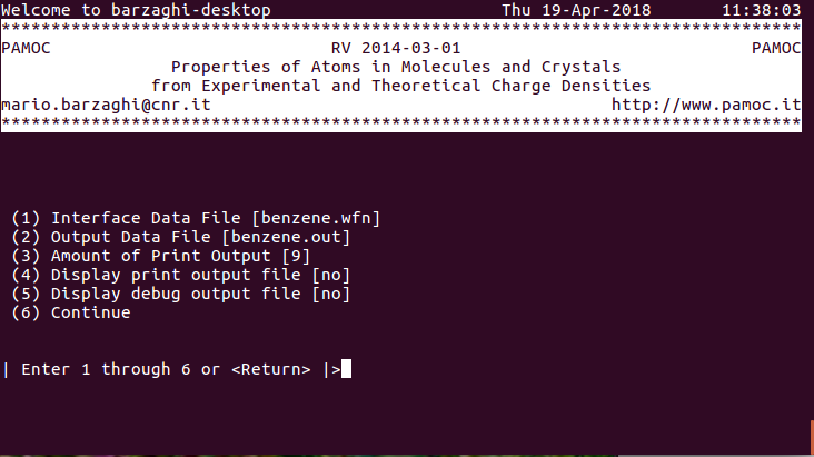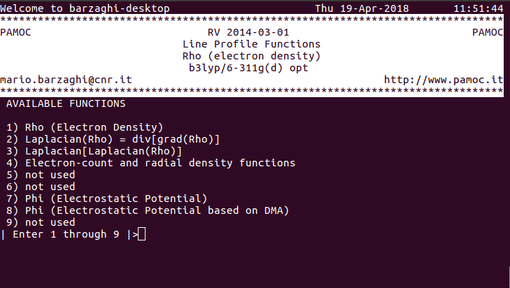
Flowchart 1. − Radial electron density profile: number of electrons in an infinitesimally thin spherical shell as a function if its radius.

(1)

(subroutine
Screen000)
choose
item 6
⇓

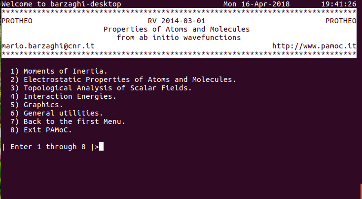
(2)

(subroutine
Screen000)
choose
item 5
⇓

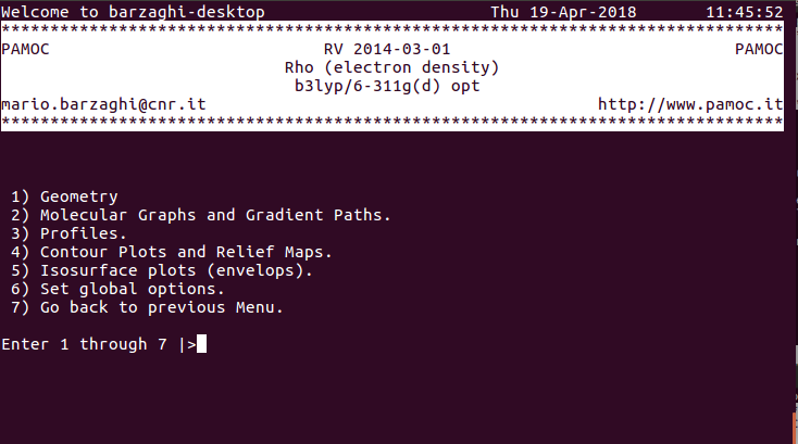(3)

(subroutine
Screen500)
choose
item 3
⇓

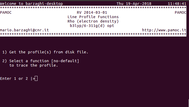
(4)

(subroutine
Screen530)
choose
item 2
⇓

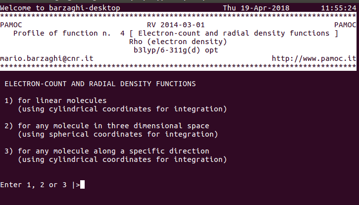
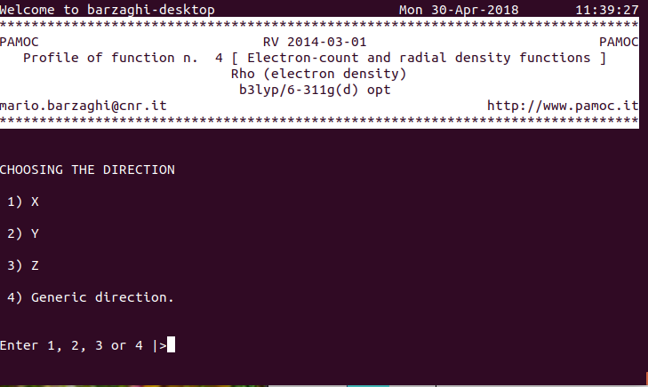
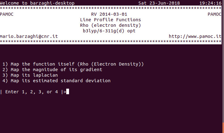
(5)

(subroutine
Screen134)
choose
item 4
⇓

(6)

(subroutine
Screen530)
choose
item 2
⇓

(7)

(subroutine
Screen530)
choose
item 2
⇓

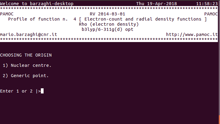
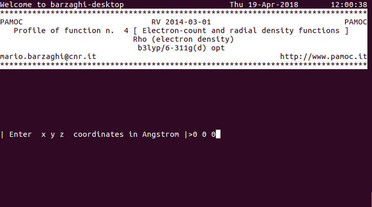
(8)

(subroutine
Screen530)

enter
the cartesian
coordinates of
the center of the
spherical shell
⇓

radial density and electron-count function of benzene

Figure 1. − The electron density, g(r), in a spherical shell volume element of infinitesimal thickness, and the electron-count function, G(r), are reported for the benzene molecule as a function of the radius r of the spherical shell, whose origin is the symmetry center of the molecule. Units are e⋅bohr⁻¹ and e, respectively.
Dashed vertical lines mark the position of carbon (r_C = 2.6338 bohr) and hydrogen (r_H = 4.6851 bohr) atoms with respect to the center of the spherical shell.

Flowchart 1. − Radial electron density profile: number of electrons in an infinitesimally thin spherical shell as a function if its radius.

It is clear from the asympotic value of the electron count function G(r) in Figure 1, as well as from the numerical results reported in the print-output file (see Section 4), that the presence of cusps at the nuclear centres destroys the accuracy of the numerical procedure used. In the example of Figure 1, the number of electrons in benzene is overestimated by 4.31 e (about 10%).

The error is even higher if the center of the spherical shell is located at a nuclear centre (screen 7, option 1, Flowchart 1), like a carbon atom (Figure 2a, error = 15.41 e or 36.7%) or an hydrogen atom (Figure 2b, error = 54.42 e or 130%).

Figure 2. − The electron density, g(r), in a spherical shell volume element of infinitesimal thickness, and the electron-count function, G(r), are reported for the benzene molecule as a function of the radius r of the spherical shell. (a) The spherical shell is centered on atom C1. (b) The spherical shell is centered on atom H1. Units are e⋅bohr⁻¹ and e, respectively.

From the examples above (Figures 1 and 2), it appears that the radial electron density of a molecular system is strongly dependent on the origin of the spherical shell, and can be of some interest only if the origin is placed in some special point, like a center of symmetry (Figure 2). On the other hand, it is particularly suited to describe the electron density of an isolated atom.

2. - Planar electron density profile.

The planar electron density at a given point on a line is the number of electrons in a plane perpendicular to that line in that point. Its units are e⋅bohr⁻¹.

To obtain the profile of this density along the line we'll follow the steps outlined in Flowchart 1 up to the screen number 6, where we will choose the option number 3 and proceed as shown below in Flowchart 2:

Flowchart 2. − Planar electron density profile: number of electrons in a plane perpendicular to a given line as a function of the intersection point with the line. Steps 1-5, not reported in this flowchart, are the same of Flowchart 1.

(6)

(subroutine
Screen530)
choose
item 3
⇓

(7)

(subroutine
Screen530)
choose
item 3
⇓

Figure 3. − The electron density, g(r), in a plane perpendicular to the direction r along the molecular axis H1−C1−−−C4−H4, and the electron-count function, G(r), are reported for the benzene molecule as a function of the position r of the orthogonal plane along the molecular axis. Units are e⋅bohr⁻¹ and e, respectively.
Red and white circles mark the position of atoms (or their projection) on the molecular axis.

On the other hand, choosing option number 1 or 2 on screen number 7 in Flowchart 2, yields the following graph

Figure 4. − The electron density, g(r), in planes parallel to the molecular plane, and the electron-count function, G(r), are reported for the benzene molecule as a function of the position r along the direction orthogonal to the molecular plane in its center. Units are e⋅bohr⁻¹ and e, respectively.

The error in the electron count is still influenced by the presence of cusps on nuclear centres, but to a lesser extent than the integration on the unit sphere. In fact, it is underestimated by 0.5 electrons (1.20%) in the case of Figure 3, and by 3.4 electrons (8.12%) in the case of Figure 4, respectively.

3. - Position electron density profile.

The position electron density at a given point in 3-D space is the number of electrons contained in an infinitesimally small volume at that point. Its units are e⋅bohr⁻³.

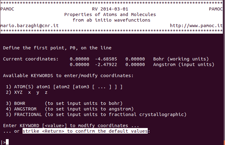
The electron density values at a number of points along a line in 3-D space provide an electron density profile along that line. It can be obtained by selecting the option number 1 on the screen number 5 in Flowchart 1, and going through the steps shown in Flowchart 3:

Flowchart 3. − (Volumetric or position) electron density profile: number of electrons contained in an infinitesimally small volume as a function of the position of the volum element. Steps 1-4, not reported in this flowchart, are the same of Flowchart 1.

(5)

(subroutine
Screen134)
choose
item 1
⇓

(6)

(subroutine
Screen134)
choose
item 1
⇓

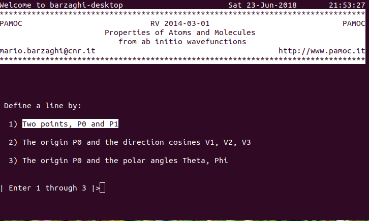(7)

(subroutine
Screen3)
choose
item 1
⇓

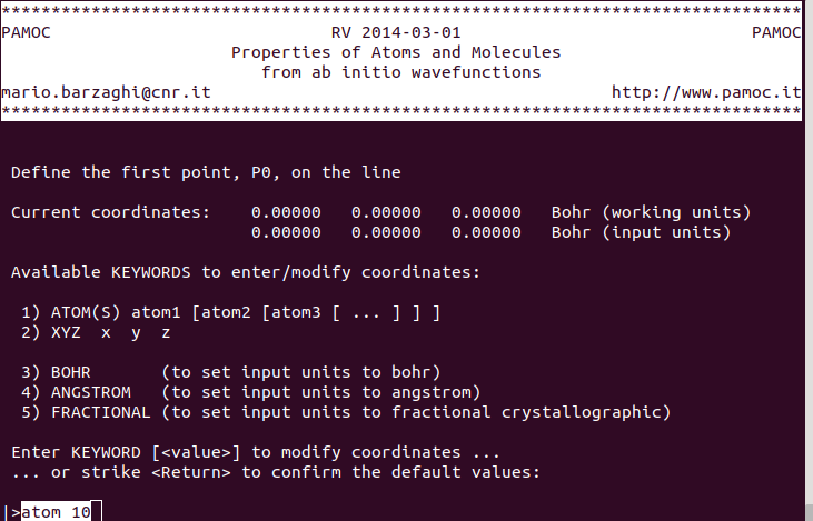
(8)

(subroutine
Screen2)

at the prompt
enter
“atom 10”
for P0
⇓

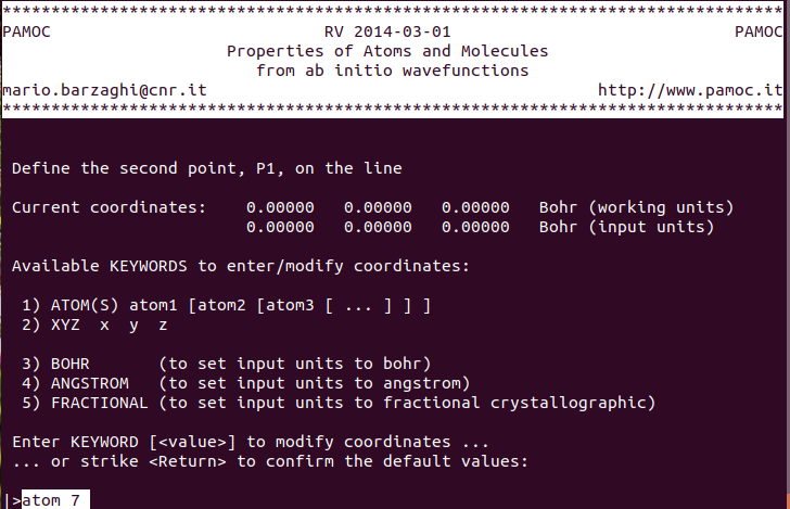
(9)

(subroutine
Screen2)

confirm
striking
“RETURN”
⇓

(10)

(subroutine
Screen2)

at the prompt
enter
“atom 7”
for P1
⇓

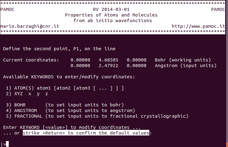(11)

(subroutine
Screen2)

confirm
striking
“RETURN”
⇓

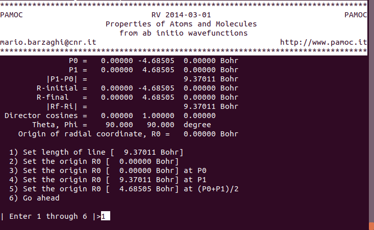
(12)

(subroutine
Screen3)
choose
item 1
⇓

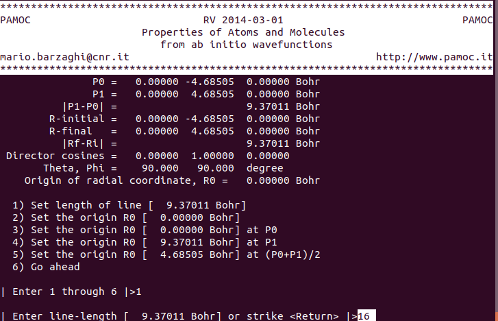(13)

(subroutine
Screen3)

enter “16”
for line-length
(bohr)
⇓

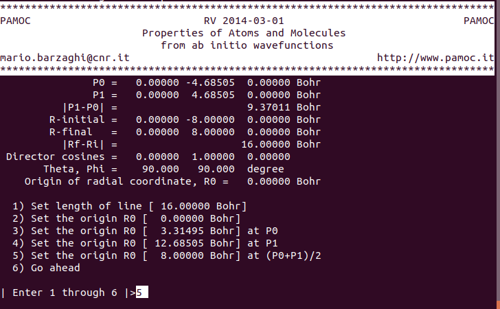
(14)

(subroutine
Screen3)

choose
item 5
⇓

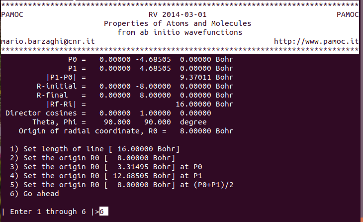(15)

(subroutine
Screen3)

choose
item 6
⇓

Figure 5. − Profile of the electron density, ρ(r), along a line containing the bonds H₁−C₁ and C₄−H₄ in the benzene molecule. The peaks are located at nuclear centers. Units are e⋅bohr⁻³.

The profiles in Figures 3 and 5 have some analogies as well as significant differences. Both figures describe the trend of the electron density along a given direction, but the values shown in Figure 5 refer to the electron density at each point of the space along that direction, while those shown in Figure 3 give the value of the total electron density in the plane perpendicular to the given direction.

4. - Output of 1-D electron density profiles

The graphs of Figures 1-5 are not produced directly by the PAMoC-TUI. Instead the latter provides numerical results in the form of a block data, which is part of the print-output file. The block data (shown in the box below) can be extracted from the print-output file and then read by GRACE.[L2"Grace (plotting tool)",
Wikipedia, The Free Encyclopedia, L3GRACE website], a free 2D graph plotting tool, for visualization. All Figures 1-5 have been obtained using GRACE. The block data reported in the box below was used to generate Figure 1.

[ … … … ] The following block data contains: - column 1: index; - column 2: r value (bohr, radius of the spherically averaged atom); - column 3: spherically averaged electron density in an infinitesinal volume element at point r (e/bohr^3); - column 4: radial electron density [i.e. electron density in a spherical shell volume element of infinitesimal thickness and radius r] (e/bohr) - column 5: electron count function (e); <-cut-here-> TOP OF BLOCK DATA FILE FOR GRACE 2D PLOTTING PROGRAM <-cut-here-> 1 0.000000 0.266737 0.000000 0.000000 2 0.010000 0.266771 0.000027 0.000000 3 0.020000 0.266873 0.000107 0.000001 4 0.030000 0.267042 0.000240 0.000004 5 0.040000 0.267280 0.000428 0.000008 6 0.050000 0.267586 0.000669 0.000015 7 0.060000 0.267959 0.000965 0.000024 8 0.070000 0.268401 0.001315 0.000038 [ … … … ] 1294 12.930000 0.000000 0.000000 46.311961 1295 12.940000 0.000000 0.000000 46.311961 1296 12.950000 0.000000 0.000000 46.311961 1297 12.960000 0.000000 0.000000 46.311961 1298 12.970000 0.000000 0.000000 46.311961 1299 12.980000 0.000000 0.000000 46.311961 1300 12.990000 0.000000 0.000000 46.311961 1301 13.000000 0.000000 0.000000 46.311961 <-cut-here-> END OF BLOCK DATA FILE FOR GRACE 2D PLOTTING PROGRAM <-cut-here-> 1D grid of 1301 data points saved on file: pamoc.g1d

Using GRACE allows the user to change visualization of data as desired. However, as indicated by the last line in the box extracted from the print-output file (see above), the PAMoC-TUI also generates a CUBE file,[L1CUBE File Format
(PAMoC Manual)] which contains the 1-D electron density profile. The default name of the CUBE file, is pamoc.g1d, but the user is allowed to change it by entering a new filename at the prompt in the following screen:

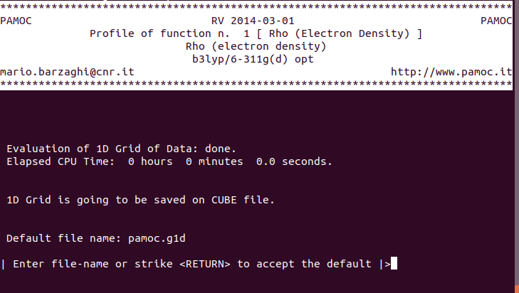(subroutines
Screen530
and
get_file)

which is always presented as soon as calculation of the 1-D electron density profile is done.

1-D electron density profiles

1. - Radial electron density profile

2. - Planar electron density profile.

3. - Position electron density profile.

4. - Output of 1-D electron density profiles

References

Links